Note:

The documentation for Classical Shadows in Mitiq is still under construction. This users guide will change in the future.

What is the theory behind Classical Shadow Estimation#

Investigating an unknown quantum system’s properties is essential in quantum computing. Quantum Tomography enables a thorough classical description of a quantum state but demands exponentially large data and an equal number of experiments. Its alternative, Shadow Tomography, requires fewer computations but presupposes the capacity to perform entangling measurements across various state copies, involving exponentially large quantum operations. This section introduces an efficient alternative that constructs an approximate classical depiction of a quantum state with minimal state measurements.

1. Classical Shadow#

The “classical shadow” technique, as proposed by [16], offers an innovative approach to quantum state approximation. This method is particularly advantageous for predicting the properties of complex, large-scale quantum systems as it requires exponentially fewer measurements. In quantum theory, the quantities of interest are often linear functionals of the quantum state \(\rho\), such as the expectation values \(o_i\) of a set of self-adjoint operators \(\{O_i\}_{i}\):

(1)#\[\begin{equation} o_i=\mathrm{Tr}(O_i \rho),\qquad i\in\mathbb{N}^+,~~ 1\leq i\leq M. \end{equation}\]

Rather than striving for a comprehensive classical description of a many-body quantum state [18]—a task that is practically challenging due to the exponentially large quantities of required classical data—this method only demands a size of \(N\) “classical shadow” to predict arbitrary \(M\) linear functions \(\mathrm{Tr}(O_i \rho)\) up to an additive error \(\epsilon\), given that

(2)#\[\begin{equation} N\geq \mathcal{O}(\epsilon^{-2}\log M\max_i \parallel O_i \parallel^2_{\mathrm{shadow}}). \end{equation}\]

In the context of an \(n-\)qubit system, where \(\rho\) is an unknown quantum state residing in a \(2^n\)-dimensional Hilbert space, the procedure of performing classical shadow involves extracting information from the state through repeated measurements. This process involves applying a random unitary selected from a randomly fixed ensemble \(\mathcal{U}\in U(2^n)\) to rotate the state \(\rho\rightarrow U^\dagger \rho U\), performing a computational-basis(\(Z\)-basis) measurement, and storing a classical description \(U^\dagger |\hat{b}\rangle\langle\hat{b}| U\). After the measurement, the inverse of \(U\) is applied to the resulting computational basis state, collapsing \(\rho\) to

(3)#\[\begin{equation} U^\dagger|\hat{b}\rangle\langle\hat{b}| U\qquad \mathrm{where} \qquad \mathrm{Pr}[\hat{b}=b]=\langle b|U\rho U^\dagger|b\rangle. \end{equation}\]

This random snapshot contains valuable information about \(\rho\) in expectation:

(4)#\[\begin{equation} \mathbb{E}[U^\dagger |\hat{b}\rangle\langle\hat{b}|U]=\sum_{b\in\{0,1\}^{\otimes n}}\mathrm{Tr}_{(1)}\left(\rho_{(1)}\mathbb{E}_{U\sim U(2^n)}[(U|b\rangle\langle b|U^\dagger)^{\otimes 2}]\right)=\mathcal{M}(\rho) \end{equation}\]

where the trace is only taken on one of the copies in the tensor product, and the expectation in the first expression has the form \(\mathbb{E}(\cdot)=\int_{U\in\mathcal{U}}d\mu(U)\;\langle b|U^\dagger\rho U|b\rangle(\cdot)\). For any unitary ensemble \(\mathcal{U}\), the expected value of the outer product of the classical snapshot corresponds to the operation of the quantum channel \(\mathcal{M}\) on the quantum state \(\rho\). This is indeed a depolarizing channel, as the middle portion of (4) transfigures into a blend of identity and a swap operator, based on Schur’s Lemma [19], when taking the Haar average of \(\mathcal{G}=U(d)\) group:

(5)#\[\begin{equation} \int_{\mathcal{G}\sim U(d)}~d\mu(\mathcal{G})(U|b\rangle\langle b|U^\dagger)^{\otimes 2}=\frac{\mathbb{I}+X}{d(d+1)}~~ \Rightarrow~~ \mathcal{M}(A)=\sum_{b\in\{0,1\}^{\otimes n}}\frac{\mathrm{Tr}(A)\mathbb{I}+(A)}{2^n(1+2^n)} = \mathcal{D}_{(2^n+1)^{-1}}(A). \end{equation}\]

Thus, the quantum channel \(\mathcal{M}\) is a depolarizing channel \(\mathcal{D}_p\) with \(p=\frac{1}{2^n+1}\). It is easy to solve for the inverted map \(\mathcal{M}^{-1}(\cdot)=[(2^n +1)-\mathbb{I}\cdot\mathrm{Tr}](\cdot)\), which is indeed unitary, however, not CP, so it is not a physical map as expected.

If the measurements we sample from are tomographically complete, then the protocol \(\mathcal{M}\) defines an invertible linear transformation \(\mathcal{M}^{-1}\), which may not be a quantum channel, since it is not CP, which means that it could not be performed in the lab. But it will only be performed on the classical data stored in a classical memory. If we apply \(\mathcal{M}\) to all the snapshots, the expected value of these inverted snapshots aligns with the density operator as defined by the protocol,

(6)#\[\begin{equation}\hat{\rho}=\mathcal{M}^{-1}\left(U^\dagger|\hat{b}\rangle\langle\hat{b}|U\right) \end{equation}\]

which has been named a single copy of classical shadow. Repeating this procedure \(N\) times results in an array of \(N\) independent classical snapshots of \(\rho\):

(7)#\[\begin{equation} S(\rho,\; N)=\big\{\hat{\rho}_1=\mathcal{M}^{-1}\left(U_1^\dagger |\hat{b}_1\rangle\langle\hat{b}_1| U_1\right),\dots,\mathcal{M}^{-1}\left(U_N^\dagger |\hat{b}_N\rangle\langle\hat{b}_N| U_N\right)\big\} \end{equation}\]

To estimate the expectation value of some observable, we simply replace the unknown quantum state \(\rho\) with a classical shadow \(\hat{\rho}\). Since classical shadows are random, this produces a random variable that yields the correct prediction in expectation:

(8)#\[\begin{equation} \hat{o}_i = \mathrm{Tr}(O_i\hat{\rho})\qquad\mathrm{obeys}\qquad \mathrm{Tr}(O_i\rho)\equiv \mathbb{E}[\hat{o}_i],\qquad~~~~ 1\leq i\leq M. \end{equation}\]

One can prove that a single classical shadow (6) can correctly predict any linear function in expectation, by taking average over the repeatedly \(N\) independent classical shadows (7),

(9)#\[\begin{equation} \hat{o}_i(N)=\mathbb{E}_{j\in N}(\hat{o}_i^{(j)}\hat{\rho}_j) \end{equation}\]

Actually, in practice, we achieve an acceptable failure probability of estimation with the statistical method of taking an average called “median of means”.

(10)#\[\begin{equation} \hat{o}_i(N,K):=\mathrm{median}\{\hat{o}_i^{(1)},\cdots,\hat{o}_i^{(K)}\}~~\mathrm{where}~~\hat{o}_i^{(j)}=N^{-1}\sum_{k=N(j-1)+1}^{Nj}\mathrm{Tr}(O_i\hat{\rho}_k),\qquad \forall~1\leq j\leq K\nonumber \end{equation}\]

The general form of the shadow norm is not clear and depends on the ensemble \(\mathcal{U}\) from which we sampled the unitaries, but there are special cases:

(11)#\[\begin{equation} \mathcal{U}=\mathrm{CL}(2^n):\qquad ~~~~ \parallel O \parallel_{\mathrm{shadow}}\leq 3\mathrm{Tr}[O^2]; \end{equation}\]

(12)#\[\begin{equation} \mathcal{U}=\mathrm{CL}(2)^n:\qquad \parallel O \parallel_{\mathrm{shadow}}\leq 4^{w}\parallel O \parallel^2,\qquad O\mathrm{~acting~on~}w\mathrm{~qubits} \end{equation}\]

The random Clifford measurement (11) involves the uniform random application of an element from the Clifford group to the state. These elements can be classically described. Afterward, the measurement is taken in a computational basis. In the context of random Clifford measurements, the shadow norm is equivalent to the Hilbert norm– specifically, the \(L_2\) norm. As a result, a large collection of (global) observables with a bounded Hilbert-Schmidt norm can be predicted efficiently. In this case based on (5), a snapshot(6) would take the form

(13)#\[\begin{equation} \hat{\rho}=(2^n+1)U^\dagger|\hat{b}\rangle\langle\hat{b}|U -\mathbb{I} \end{equation}\]

On the other hand, a random Pauli measurement (11) means that for each qubit, we randomly decide to measure the Pauli operators. The shadow norm, in this situation, correlates with the operator norm. This guarantees the accurate prediction of many local observables from only a much smaller number of measurements. In this case, the unitary could be represented by the tensor product of all qubits, so it is with the state \(|\hat{b}\rangle\in\{0,1\}^{\otimes n}\), i.e. \(U^\dagger|\hat{b}\rangle=\bigotimes_{i\leq n}U_i|\hat{b}_i\rangle\). Therefore, based on (5), a snapshot(6) would takes the form:

(14)#\[\begin{equation} \hat{\rho}=\bigotimes_{i=1}^{n}\left(3U_i^\dagger|\hat{b}_i\rangle\langle\hat{b}_i|U_i-\mathbb{I}\right),\qquad|\hat{b_i}\rangle\in\{0,1\}. \end{equation}\]

The Clifford measurement requires the depth of the circuit to grow linearly with system size, which is not currently feasible for large systems, which is why only the local (Pauli) measurement is implemented in Mitiq in the current stage. However, it is worth noting that this method involves an intermediate step of scrambling the circuits and combining the local and global measurement [20].

2. Robust Shadow Estimation#

The robust shadow estimation approach put forth in [17] exhibits noise resilience. The inherent randomization in the protocol simplifies the noise, transforming it into a Pauli noise channel that can be characterized relatively straightforwardly. Once the noisy channel \(\widetilde{\mathcal{M}}\) is characterized, it is incorporated into the channel inversion \(\widetilde{\mathcal{M}}^{-1}\), resulting in an unbiased state estimator. The sampling error in the determination of the Pauli channel contributes to the variance of this estimator.

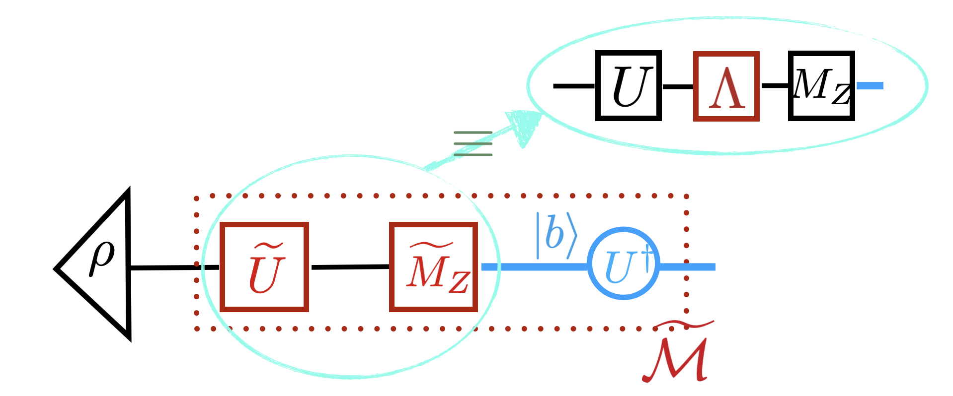
The source of the noise is the noisy quantum process, involving the application of the adjoint action of the unitary sampled randomly from \(\mathcal{U}\), and the computational (\(Z\)-) basis measurement \(M_Z\). The noisy channel (assumed to be CPTP), denoted by \(\widetilde{U}\) and \(\widetilde{M}_Z\), can be decomposed into a noiseless channel and a noisy channel \(\widetilde{U}\widetilde{M}_Z=U\Lambda_{U}\Lambda_z{M}_Z\) without loss of generality. The noise in the circuit is assumed to be gate-independent, time-invariant, and Markovian noise, which facilitates a robust calibration strategy. This leads to the noisy channel \(\Lambda_{U}\Lambda_z\equiv \Lambda\).

The noise in the quantum processing prevents the inversion of the original quantum channel from reversing the process. This necessitates a calibration process. Distinguishing \(\Lambda_U\) from the unknown state \(\rho\) is generally infeasible, so the noisy quantum channel \(\widetilde{\mathcal{M}}\) must be characterized using a known state, such as \(\mathbf{|0\rangle}:= |0\rangle^{\otimes n}\), to calibrate the noise. This preparation of \(|0\rangle\) is also susceptible to noise, but it provides high fidelity in actual estimation.

2.1 Pauli Twirling of quantum channel and Pauli Fideltiy#

The classical shadow estimation employs a quantum channel, which is subsequently inverted. This operation essentially embodies a Pauli twirling. Within this framework, \(\mathcal{G}\) represents a subset, to be further identified within the unitaries in \(U(d)\). Moreover, \(\mathcal{U}\) personifies the PTM representation of \(U\). As \(\mathcal{G}\) takes the form of a group, the PTMs \({\mathcal{U}}\) evolve into a representation of \(\mathcal{G}\). The implementation of Schur’s Lemma facilitates the direct computation of the precise form of \(\widehat{\mathcal{M}}\) when the noisy channel \(\Lambda\), representing both the gate noise \(\mathcal{U}\) and the measurement noise \(\mathcal{M}_Z\), is integrated:

(15)#\[\begin{equation} \widehat{\mathcal{M}} = \mathbb{E}_{\mathcal{G}}[\mathcal{U}^\dagger\mathcal{M}_z\Lambda\mathcal{U}] = \sum_{\lambda}\hat{f}_\lambda\Pi_\lambda,\qquad \hat{f}_\lambda:=\frac{\mathrm{Tr}(\mathcal{M}_z\Lambda\Pi_\lambda)}{\mathrm{Tr}(\Pi_\lambda)} \end{equation}\]

where \(\mathbb{R}_{\mathcal{G}}\) symbolizes the set of irreducible sub-representations of the group \(\mathcal{G}\). The total number of these coefficients is related to the number of irreducible representations in the PTM representation of the twirling group \(\mathcal{G}\). \(\Pi_\lambda\), on the other hand, denotes the corresponding projector onto the invariant subspace, which exhibits pairwise orthogonality.

When the subgroup of \(U(d)\) is the local Clifford group \(Cl_2^{\otimes n}\), the projection onto irreducible representation can be decomposed into projections acting on each qubit: \(\Pi_b=\bigotimes_{i=1}^n\Pi_{b_i}\), where \(b_i\in\{0,1\}\) specifies the measurement basis state. Here is the equation for this relationship:

(16)#\[\begin{equation} \Pi_{b_i}=\left\{ \begin{array}{ll} |\sigma_0\rangle\!\rangle\langle\!\langle\sigma_0|& b_i=0 \\ \mathbb{I}- |\sigma_0\rangle\!\rangle\langle\!\langle\sigma_0|& b_i = 1 \end{array}\right. \end{equation}\]

Therefore, the \(n\)-qubit local Clifford group has \(2^n\) irreps.

The expansion coefficients of the twirled channel, \(\{\hat{f}_{b}\}_b\), are referred to as the Pauli fidelity. Being twirled by the local Clifford group, the channel \(\widehat{M}\) becomes a Pauli channel that is symmetric among the \(x, \;y,\; z\) indices. This sequence results in a computational basis measurement outcome \(|b\rangle\) interpreted in terms of bitstrings b: \(\{0,1\}^{n}\). Subsequently, compute the single-round Pauli fidelity estimator \(\hat{f}^{(r)}_b = \langle\!\langle b|\mathcal{U}|P_b\rangle\!\rangle\) for every possible measurement outcome bitstring b: \(\{0,1\}^n\), with \(|P_b\rangle\!\rangle=\prod_i|P_{Z}^{b_i}\rangle\!\rangle\).

The Pauli fidelity estimator for the local Clifford group can be computed utilizing the subsequent equation:

(17)#\[\begin{equation} \hat{f}^{(r)}_b = \prod_{i=1}^n \langle\!\langle b_i|\mathcal{U}_i|P_z^{b_i}\rangle\!\rangle \equiv \prod_{i=1}^n \langle b_i|\mathcal{U}_i P_Z^{b_i}\mathcal{U}^\dagger_i|b_i\rangle, \qquad \mathcal{U}_i\in\mathrm{CL}(2),~ b_i\in\{0,1\}. \end{equation}\]

Repeat the above step for \(R = NK\) rounds. Then the final estimation of \(f_z\) is given by a median of means estimator \(\hat{f}_m\) constructed from the single round estimators \(\{\hat{f}_m^{(r)}\}_{1\leq r\leq R}\) with parameter \(N, \;K\): calculate \(K\) estimators each of which is the average of \(N\) single-round estimators \(\hat{f}\), and take the median of these \(K\) estimators as our final estimator \(\hat{f}\). In formula,

(18)#\[\begin{eqnarray} &\bar{f}^{(k)}=\frac{1}{N}\sum_{r=(K-1)N+1}^{KN} \hat{f}^{(r)}\\ & \hat{f} = \mathrm{median}\{\bar{f}^{(1)},\cdots\bar{f}^{(K)}\}_{1\leq k\leq K} \end{eqnarray}\]

The number of \(\{f_m\}\) is related to the number of irreducible representations in the PTM[1] representation of the twirling group. When the twirling group is the local Clifford group, the number of irreducible representations is \(2^n\).

2.2 Noiseless Pauli Fidelity — Ideal Inverse channal vs Estimate Noisy Inverse channel#

One could check that in the absence of noise in the quantum gates (\(\Lambda\equiv\mathbb{I}\)), the value of the Pauli fidelity \(\hat{f}_{b}^{\mathrm{ideal}}\equiv \mathrm{Tr}(\mathcal{M}_z \Pi_b)/\mathrm{Tr}\Pi_b = 3^{-|{b}|}\), where \(|b|\) is the count of \(|1\rangle\) found in z-eigenstates \(|b\rangle:=|b_i\rangle^{\otimes n}\).

When the noisy channel \(\widehat{\mathcal{M}}\) is considered, the inverse of the noise channel \(\widehat{\mathcal{M}}^{-1}\) can be obtained by:

(19)#\[\begin{equation} \widehat{\mathcal{M}}^{-1}=\sum_{b\in\{0,1\}^{\otimes n}}\hat{f}_b^{-1}\Pi_b \end{equation}\]

After the above steps, we can preform robust shadow calibration as we did in the standard classical shadow protocol. The only difference is we perform the inverse channel replaced by the calibrated version \(\widehat{\mathcal{M}}^{-1}\). One can see that the inverse of the noisy channel \(\mathrm{Tr}(\mathcal{M}_z \Pi_b)\) is different from the one used in the classical shadow protocol by their difference on the Pauli fidelity \(\hat{f}_b^{-1}\). The set of noise parameters \(\{f_\lambda\}_{\lambda}\) corresponds to the number of irreducible representations of \(\mathcal{G}\), called Pauli fidelity. When the unitaries are sampled from local Clifford group, the Pauli fidelities can be computed with the following formula:

Therefore, the classical shadow combined with the calibration procedure will, first, estimate the noise channel \(\widetilde{\mathcal{M}}\) of Eq. (14) via the calibration procedure, and then use the \(\widetilde{\mathcal{M}}\) estimator as the input parameter, \(\mathcal{M}\rightarrow\widetilde{\mathcal{M}}\) of the classical shadow to predict any properties of interest (referred to as the estimation procedure).