What additional options are available when using ZNE?

In the introductory section How do I use ZNE?, we used the function execute_with_zne() to evaluate error-mitigated expectation values with zero-noise extrapolation. Beyond the positional arguments (circuit, executor and observable) that are common to all error mitigation techniques, one can use additional keyword arguments for optional settings as shown in next code snippet:

from mitiq import zne

zne_value = zne.execute_with_zne(
    circuit,
    executor,
    observable,
    scale_noise = <"noise scaling method imported from zne.scaling">,
    factory = <"extrapolation Factory imported from zne.inference">,
    num_to_average = <"number of repeated evaluations for each noise-scaled circuit">,
)

The three main options are scale_noise, factory and num_to_average.

• The option scale_noise can be used to select a noise scaling method. More details are explained below.

• The option factory can be used to select an extrapolation method. More details are explained below.

• The option num_to_average can be used to average over multiple evaluations of each noise-scaled expectation value.

In the next sections we explain in more details how noise scaling and extrapolation methods are represented in Mitiq and how they can be applied in practice.

Noise scaling functions

To apply ZNE, we need to effectively increase the noise acting in a quantum computation. Instead of directly controlling the physical backend, Mitiq achieves this task by digital noise scaling, i.e., with circuit manipulations that indirectly increase the effect of noise but keep the circuit logic unchanged. More details on digital ZNE can be found in What is the theory behind ZNE?

In Mitiq a noise scaling method is represented by a noise scaling function that takes as input a circuit and a real scale_factor and returns a scaled_circuit. For a noiseless backend, scaled_circuit has the same effect as circuit. For a noisy backend, scaled_circuit is more sensitive to errors depending on the magnitude of scale_factor.

As discussed previously in How do I use ZNE?, the two available methods to scale noise are by inserting unitaries or by inserting layers of identity gates. Note that the number of layers inserted are different for the two methods even if they have the same scale factor greater than 1.

Unitary Folding

Mitiq provides several noise scaling functions for the repeated application of the unitary folding technique. In this technique regardless of the unitary folding function used, a unitary \(G\) is mapped as follows:

\[G \longrightarrow G G^\dagger G.\]

If this is applied to individual gates of a circuit, we call it local folding. If \(G\) is the entire circuit, we call it global folding.

The Mitiq function for global folding is:

• fold_global().

The Mitiq functions for local folding are:

• fold_gates_at_random();

• fold_gates_from_left();

• fold_gates_from_right();

• fold_all().

There are multiple functions for local folding since it can be applied to the gates of a circuit according to different orderings: at random, from left (starting from the initial gates), from right (starting from the final gates), etc.. For more details on folding functions, we suggest to click on the functions listed above and check the associated API docs.

If not specified by the user, the default noise scaling method in Mitiq is fold_gates_at_random(). Custom noise-scaling functions can also be defined by the user, as shown in What happens when I use ZNE ?.

Note: All scaling functions can be applied to circuits defined in any supported frontend. For example, in the next code cells we use Cirq to represent quantum circuits.

The special case of odd integer scale factors

For any noise scaling function, if scale_factor is equal to 1, the input circuit is unchanged and it is subject to the base noise of the backend.

Both local and global folding, if applied uniformly to all the gates of circuit, produce a scaled_circuit that has 3 times more gates than the input circuit. This corresponds to the scale_factor=3 setting. For example:

import cirq
from mitiq import zne

# Get a circuit to fold
qreg = cirq.LineQubit.range(2)
circuit = cirq.Circuit(cirq.ops.H.on(qreg[0]), cirq.ops.CNOT.on(qreg[0], qreg[1]))
print("Original circuit:", circuit, sep="\n")

# Apply local folding
scaled_circuit = zne.scaling.fold_gates_at_random(circuit, scale_factor=3)
print("Locally folded circuit:", scaled_circuit, sep="\n")

# Apply global folding
scaled_circuit = zne.scaling.fold_global(circuit, scale_factor=3)
print("Globally folded circuit:", scaled_circuit, sep="\n")

Original circuit:
0: ───H───@───
          │
1: ───────X───
Locally folded circuit:
0: ───H───H───H───@───@───@───
                  │   │   │
1: ───────────────X───X───X───
Globally folded circuit:
0: ───H───@───@───H───H───@───
          │   │           │
1: ───────X───X───────────X───

The same trick can be generalized to any odd integer scale_factor. In this case, folding functions apply the mapping \(G \longrightarrow G (G^\dagger G)^{({\rm scale\_factor} - 1)/2}\). For example:

num_gates = len(list(circuit.all_operations()))
for scale_factor in [1, 3, 5, 7]:
    scaled_circuit = zne.scaling.fold_global(circuit, scale_factor)
    scaled_num_gates = len(list(scaled_circuit.all_operations()))
    print(f"For scale_factor={scale_factor}, the number of gates was scaled by {scaled_num_gates / num_gates}")

For scale_factor=1, the number of gates was scaled by 1.0
For scale_factor=3, the number of gates was scaled by 3.0
For scale_factor=5, the number of gates was scaled by 5.0
For scale_factor=7, the number of gates was scaled by 7.0

Note: When scale_factor is an odd integer, the number of gates is scaled exactly as dictated by the value of scale_factor. In this case, since all gates are folded the same number of times, the three local folding functions fold_gates_at_random(), fold_gates_from_left() and fold_gates_from_right() have the same (deterministic) effect.

The general case of real scale factors

More generally, the scale_factor can be set to any real number larger than or equal to one. In this case, Mitiq applies additional folding to a selection of gates (for local folding) or to a final fraction of the circuit (for global folding), such that the total number of gates is approximately scaled by scale_factor. For example:

num_gates = len(list(circuit.all_operations()))
for scale_factor in [1.2, 1.4, 1.6, 1.8, 2.0]:
    scaled_circuit = zne.scaling.fold_gates_at_random(circuit, scale_factor)
    scaled_num_gates = len(list(scaled_circuit.all_operations()))
    print(f"For scale_factor={scale_factor}, the number of gates was scaled by {scaled_num_gates / num_gates}")

For scale_factor=1.2, the number of gates was scaled by 1.0
For scale_factor=1.4, the number of gates was scaled by 1.0
For scale_factor=1.6, the number of gates was scaled by 2.0
For scale_factor=1.8, the number of gates was scaled by 2.0
For scale_factor=2.0, the number of gates was scaled by 2.0

Note: As printed above, if scale_factor is not an odd integer and if the input circuit is very short, there can be a large error in the actual scaling of the number of gates. For this reason, when dealing with very short circuits, we suggest to use odd integer scale factors.

For longer circuits, real scale factors are better approximated. Indeed, when num_gates and scaled_num_gates are large integers, their ratio can take values with a more fine-grained resolution.

long_circuit = circuit * 5
num_gates = len(list(long_circuit.all_operations()))
for scale_factor in [1.2, 1.4, 1.6, 1.8, 2.0]:
    scaled_circuit = zne.scaling.fold_gates_at_random(long_circuit, scale_factor)
    scaled_num_gates = len(list(scaled_circuit.all_operations()))
    print(f"For scale_factor={scale_factor} the number of gates was scaled by {scaled_num_gates / num_gates}")

For scale_factor=1.2 the number of gates was scaled by 1.2
For scale_factor=1.4 the number of gates was scaled by 1.4
For scale_factor=1.6 the number of gates was scaled by 1.6
For scale_factor=1.8 the number of gates was scaled by 1.8
For scale_factor=2.0 the number of gates was scaled by 2.0

Folding gates by fidelity

In local folding methods, gates can be folded according to custom fidelities by passing the keyword argument fidelities. This argument should be a dictionary where each key is a string which specifies the gate and the value of the key is the fidelity of that gate. An example is shown below where we set the fidelity of all single qubit gates to be 1.0, meaning that these gates introduce negligible errors in the computation.

# Define test circuit
qreg = cirq.LineQubit.range(3)
test_circuit = cirq.Circuit((
    cirq.ops.H.on_each(*qreg),
    cirq.ops.CNOT.on(qreg[0], qreg[1]),
    cirq.ops.T.on(qreg[2]),
    cirq.ops.TOFFOLI.on(*qreg)
    
))
print("Original circuit:", test_circuit, "", sep="\n")

# Fold by fidelities
folded = zne.scaling.fold_gates_at_random(
    test_circuit, scale_factor=3, fidelities={"single": 1.0, "CNOT": 0.99, "TOFFOLI": 0.95},
)
print("Folded circuit:", folded, sep="\n")

Original circuit:
0: ───H───@───@───
          │   │
1: ───H───X───@───
              │
2: ───H───T───X───

Folded circuit:
0: ───H───@───@───@───@───@───@───
          │   │   │   │   │   │
1: ───H───X───X───X───@───@───@───
                      │   │   │
2: ───H───T───────────X───X───X───

We can see that only the two-qubit gates and three-qubit gates have been folded.

Specific gate keys override the global "single", "double", or "triple" options. For example, the dictionary fidelities = {"single": 1.0, "H": 0.99} sets all single qubit gates to fidelity one except the Hadamard gate.

A full list of string keys for gates can be found with help(fold_method) where fold_method is a valid local folding method. Fidelity values must be between zero and one.

Folding gates by layer

Circuit debugging techniques, as proposed in Calderon et al. Quantum (2023) [3], utilize the ability to apply layerwise folding of a circuit.

A quantum circuit \(C\) may be represented as a series of \(d\) layers. Each layer \(L\) contains one or more quantum gates acting concurrently on an \(n\)-qubit system:

\[ C = L_d L_{d-1} \cdots L_2 L_1. \]

The \(i\)-inverse operation of a circuit \(C\) is defined as

\[ C^{(i)} = L_d \cdots L_{i+1} [L_i L_i^{-1} L_i] L_{i-1} \cdots L_1 \]

where we refer to \(L_i\) as the target layer and \(L_i^{-1}\) as the inverse target layer. The inverse target layer is composed of gates that would invert the gates in the target layer.

One can perform \(m\) such inversions on a quantum circuit as well. A multiple \(i\)-inversion is defined as

\[ C^{(i)} = L_d \cdots L_{i+1} L_i \left[L_i^{-1} L_i\right]^m L_{i-1} \cdots L_1 \]

where we apply a given \(i\)-inversion \(m\) times.

For example, consider the following circuit

from mitiq.zne.scaling.layer_scaling import layer_folding

q0, q1 = cirq.LineQubit.range(2)
circuit = cirq.Circuit(
    cirq.H(q0),
    cirq.CNOT(q0, q1),
)
print(circuit)

0: ───H───@───
          │
1: ───────X───

This circuit consists of two layers (the first layer has a Hadamard gate and the second layer has a CNOT gate).

We can make use of the layer_folding() function where the argument layers_to_fold is a list of size \(d\) where each element in the list is an integer that refers to the number of times to fold the layer at index i.

As an example, we can apply a single fold only to the first layer of the circuit

print(layer_folding(circuit, [1, 0]))

0: ───H───H───H───@───
                  │
1: ───────────────X───

We can also fold specific layers a variable number of times. Here is an example of folding the first layer twice and the second layer three times.

print(layer_folding(circuit, [2, 3]))

0: ───H───H───H───H───H───@───@───@───@───@───@───@───
                          │   │   │   │   │   │   │
1: ───────────────────────X───X───X───X───X───X───X───

The layer_folding function could be used for noise diagnostics [3] or for a low-level implementation of ZNE in a similar way as shown in the next section.

To get a noise scaling function which is instead directly compatible with execute_with_zne() one can use get_layer_folding().

Identity Scaling

The goal of this technique is to insert layers of identity gates to extend the duration of the circuit, which, when used in the context of ZNE, provides a useful noise-scaling method. Mathematically, this is represented as composing identity operations after the target unitary \(G\).

\[G \longrightarrow I G\]

Here, \(G\) is a single circuit layer containing individual that can be performed simultaneously.

To use this method, call zne.scaling.identity_insertion.insert_id_layers() with both a circuit to scale, and a scale factor. Alternatively, pass it as the scale_noise argument to zne.execute_with_zne() to use it instead of the default method of fold_gates_at_random().

Integer and Real Scale Factors

When the scale factor is 1, no identity layers are inserted and circuit depth remains unchanged.

For some scale factor greater than 1, there will need to be some layers inserted non-uniformly to approach the desired scale factor. This is determined by the scale factor being an integer or a float.

• When the scale factor is an integer, identity layers are inserted uniformly after each moment in the input circuit.

• When the scale factor is a non-integer, identity layers are inserted uniformly until the closest integer less than the scale factor is achieved. Then the layers are inserted at random to achieve a value approximately close to the intended scale factor.

Example

Consider an input circuit of depth \(d\). Let \(\lambda\) be the desired scale factor, \(n\) be the number of uniformly inserted identity layers and \(s\) be the number of randomly inserted identity layers. The scaled circuit depth is then approximated as \(\lambda d \approx d(1+n) + s\).

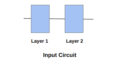
The diagram shows the two layers in the input circuit.

Using the same circuit defined previously, the original circuit depth is \(2\). If the desired scale factor is \(5\) then the new scaled circuit depth has to be \(10\) as \(5 = \frac{10}{2}\). Using above expression for \(\lambda = 1+ 4\), the number of uniformly inserted identity layers in the scaled circuit will be \(4\).

The diagram shows the uniform layers inserted in the input circuit after the initial circuit was scaled via identity insertion scaling for an integer scale factor.

If the scale factor is a non-integer greater than or equal to 1, the identity layer insertion can be described as a mix of uniform and randomly inserted layers. In some cases, achieving the exact scale factor is not possible, but this method will insert identities appropriately to closely approximate it.

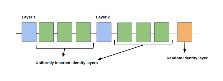
The diagram shows the uniform layers and random layer inserted in the input circuit after the initial circuit was scaled via identity insertion scaling for a real scale factor.

import cirq
from mitiq import zne

# Get a circuit to fold
qreg = cirq.LineQubit.range(2)
circuit = cirq.Circuit(cirq.ops.H.on(qreg[0]), cirq.ops.CNOT.on(qreg[0], qreg[1]))
print("Original circuit:", circuit, sep="\n")

# Apply identity scaling for uniform layers
scaled_circuit = zne.scaling.insert_id_layers(circuit, scale_factor=5)
print("Identity Scaled circuit for an integer scale factor :", scaled_circuit, sep="\n")

# Apply identity scaling for non-integer scale factor
scaled_circuit = zne.scaling.insert_id_layers(circuit, scale_factor=5.5)
print("Identity Scaled circuit for a non-integer scale factor :", scaled_circuit, sep="\n")

Original circuit:
0: ───H───@───
          │
1: ───────X───
Identity Scaled circuit for an integer scale factor :
0: ───H───I───I───I───I───@───I───I───I───I───
                          │
1: ───────I───I───I───I───X───I───I───I───I───
Identity Scaled circuit for a non-integer scale factor :
0: ───H───I───I───I───I───I───@───I───I───I───I───
                              │
1: ───────I───I───I───I───I───X───I───I───I───I───

Extrapolation methods: Factory objects

Extrapolation methods are represented in Mitiq as Factory objects. The typical tasks of a Factory are:

1. Record the result of the computation executed at the chosen noise level;

2. Determine the noise scale factor at which the next computation should be run;

3. Given the history of noise scale factors and results, evaluate the associated zero-noise extrapolation.

The Factory class has two main abstract subclasses:

• BatchedFactory representing non-adaptive extrapolation algorithms in which the noise scale factors are fixed and a batch of noise scaled circuits is measured;

• AdaptiveFactory representing adaptive extrapolation algorithms in which the choice of the next noise scale factor depends on the history of the measured results.

Specific classes derived from BatchedFactory or AdaptiveFactory represent different zero-noise extrapolation methods.

Mitiq provides a number of built-in factories, which can be found in the module mitiq.zne.inference and are summarized in the following table.

LinearFactory	Factory object implementing zero-noise extrapolation based on a linear fit.
RichardsonFactory	Factory object implementing Richardson extrapolation.
PolyFactory	Factory object implementing a zero-noise extrapolation algorithm based on a polynomial fit.
ExpFactory	Factory object implementing a zero-noise extrapolation algorithm assuming an exponential ansatz y(x) = a + b * exp(-c * x), with c > 0.
PolyExpFactory	Factory object implementing a zero-noise extrapolation algorithm assuming an (almost) exponential ansatz with a non linear exponent y(x) = a + sign * exp(z(x)), where z(x) is a polynomial of a given order.
AdaExpFactory	Factory object implementing an adaptive zero-noise extrapolation algorithm assuming an exponential ansatz y(x) = a + b * exp(-c * x), with c > 0.

In Mitiq the default extrapolation method is Richardson extrapolation with scale factors 1, 2 and 3 and corresponding to the following Factory object:

from mitiq import zne

# Default extrapolation method in Mitiq
richardson_factory = zne.inference.RichardsonFactory(scale_factors=[1, 2, 3])

Different extrapolation methods can be initialized in a similar way. For example:

# Linear fit with scale factors 1 and 3
linear_factory = zne.inference.LinearFactory(scale_factors=[1, 3])

# Polynomial fit of degree 2 with scale factors [1, 1.5, 2, 2.5, 3] .
poly_factory = zne.inference.PolyFactory(scale_factors=[1, 1.5, 2, 2.5, 3], order=2)

# Exponential fit with scale factors [1, 2, 3] assuming an infinite-noise limit of 0.5.
exp_factory = zne.inference.ExpFactory(scale_factors=[1, 2, 3], asymptote=0.5)

# Adaptive exponential fit with 5 scale factors, assuming an infinite-noise limit of 0.5.
adaptive_factory = zne.inference.AdaExpFactory(steps=5, asymptote=0.5)

Note: Richardson extrapolation is equivalent to an exact polynomial interpolation. This means that a RichardsonFactory object is equivalent to a PolyFactory with order=len(scale_factors) - 1.

Running ZNE with advanced options

To show an example, we define a circuit and an executor as shown in How do I use ZNE? but apply ZNE with advanced options.

from mitiq import benchmarks

circuit = benchmarks.generate_rb_circuits(n_qubits=2, num_cliffords=2)[0]
circuit

0: ───X^-0.5───Y^0.5───@───Y^0.5────@───Y^0.5───X─────Y^0.5───@───Y^0.5────@───Y^0.5────Y^-0.5───X^-0.5───@───X^0───────────
                       │            │                         │            │                              │
1: ───X^0──────────────@───X^-0.5───@───X^0.5───X^0───────────@───X^-0.5───@───Y^-0.5───X^0.5────Y^0──────@───Y─────X^0.5───

Typically the noise of single-qubit gates is negligible with respect to the noise of two-qubit gates. To simulate this fact, we define an executor that simulates the effect of depolarizing noise acting on two-qubit gates only.

from cirq import DensityMatrixSimulator, depolarize
from mitiq import Executor

def execute(circuit, noise_level=0.1):
    """Returns Tr[ρ |0⟩⟨0|] where ρ is the state prepared by the circuit
    executed with depolarizing noise acting on two-qubit gates.
    """
    # Replace with code based on your frontend and backend.
    noisy_circuit = cirq.Circuit()
    for op in circuit.all_operations():
        noisy_circuit.append(op)
        # Add depolarizing noise after two-qubit gates
        if len(op.qubits) == 2:
            noisy_circuit.append(depolarize(p=noise_level, n_qubits=2)(*op.qubits))

    rho = DensityMatrixSimulator().simulate(noisy_circuit).final_density_matrix
    return rho[0, 0].real

executor = Executor(execute)

In the next code cell we run ZNE with several advanced options:

• We seed the noise scaling function;

• We fold only CNOT gates using the fidelity option;

• We use a non-default extrapolation method (ExpFactory).

Note: The scope of the next code cell is not to define an optimal ZNE estimation, but to show a large number of options.

from functools import partial
import numpy as np

# Random local folding applied to two-qubit gates with a seeded random state 
random_state = np.random.RandomState(0)
noise_scaling_function = partial(
    zne.scaling.fold_gates_at_random,
    fidelities = {"single": 1.0},  # Avoid folding single-qubit gates
    random_state=random_state,  # Useful to get reproducible results
)
# Exponential fit with scale factors [1, 2, 3], assuming an infinite-noise limit of 0.5.
factory = zne.inference.ExpFactory(scale_factors=[1, 2, 3], asymptote=0.25)

zne_value = zne.execute_with_zne(
    circuit=circuit,
    executor=executor,
    observable=None,
    factory=factory,
    scale_noise=noise_scaling_function,
    num_to_average=3,
)

zne_value

0.9992706872985327

Analysis of ZNE data

Since we defined a factory with 3 scale factors and since num_to_average=3, we expect \(3 \times 3=9\) circuit evaluations. Indeed:

executor.calls_to_executor

9

The corresonding noisy results are:

executor.quantum_results

[0.67670625,
 0.67670625,
 0.67670625,
 0.5217586,
 0.52175856,
 0.5217587,
 0.3881229,
 0.3881229,
 0.3881229]

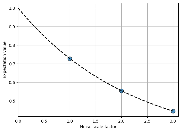
The noise scaled expectation values (averaged over num_to_average=3 raw results) are:

factory.get_expectation_values()

[0.6767062544822693, 0.5217586159706116, 0.38812288641929626]

We can also visualize the extrapolation fit:

_ = factory.plot_fit()

In this section we have shown how to run ZNE with non-default options. A lower-level usage of noise scaling methods and Factory objects is presented the next section (What happens when I use ZNE?).