What happens when I use PEA?#
PEA in Mitiq is divided into two steps: probabilistic sampling of noise-amplified circuits, and extrapolation of the corresponding expectation values. The workflow is shown in the figure below.
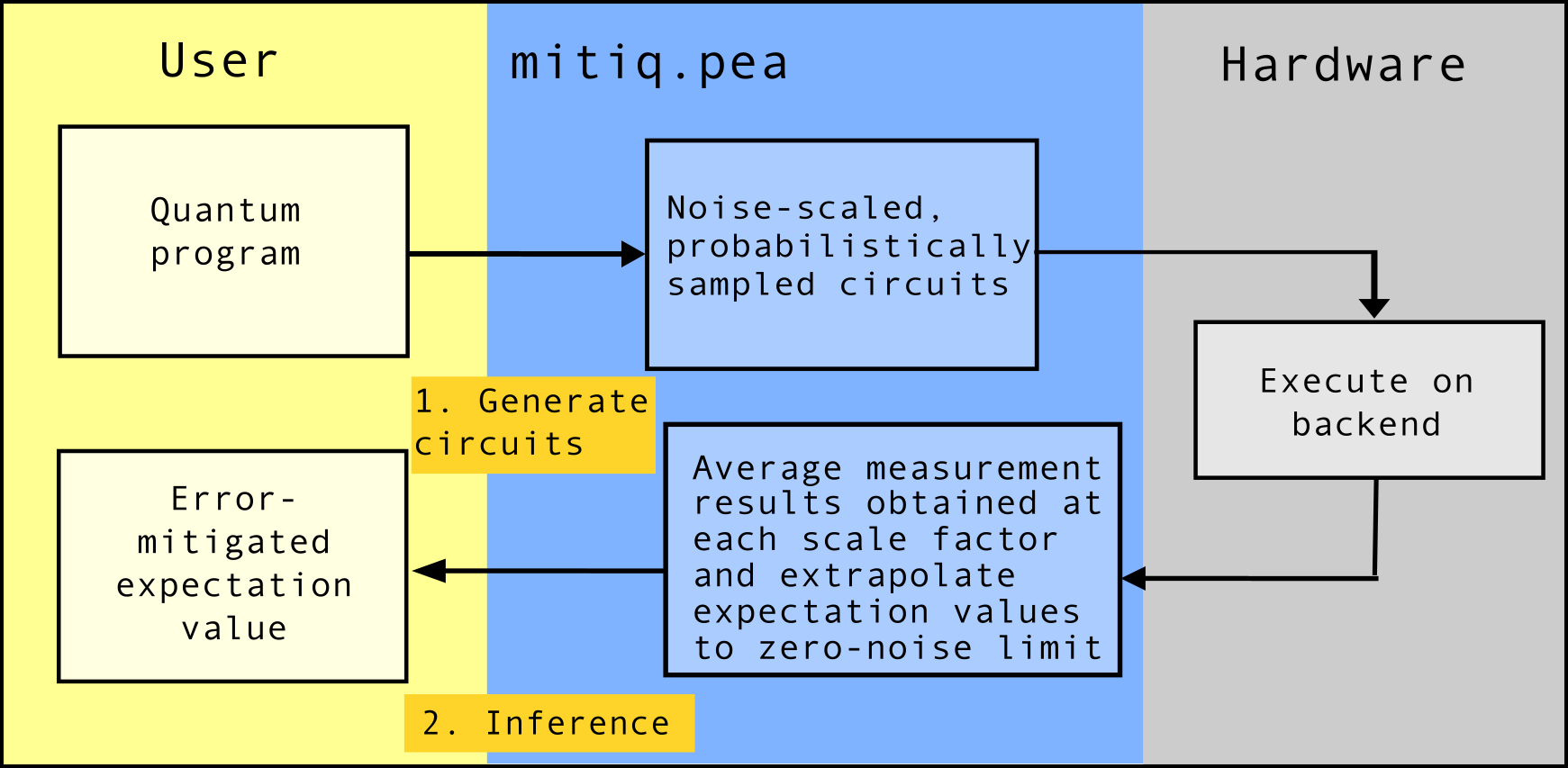
The diagram shows the workflow of the probabilistic error amplification (PEA) technique in Mitiq.#
The first step involves generating and executing noise-amplified circuits.
The user provides a
QPROGRAM(a circuit from a supported frontend).Mitiq generates lists of probabilistically sampled circuits for each noise scale factor using a noise model and baseline noise level.
Each sampled circuit is executed and its noisy expectation value recorded.
The second step involves combining the sampled results at each scale factor and extrapolating to the zero-noise limit using a ZNE-style inference method.
As demonstrated in How do I use PEA?, the function
execute_with_pea() applies both steps behind the scenes.
In the next sections, we show how to apply each step independently.
First step: generating and executing noise-amplified circuits#
Problem setup#
We define a circuit and an executor, as shown in How do I use PEA?.
from mitiq import benchmarks
from cirq import DensityMatrixSimulator, depolarize

circuit = benchmarks.generate_rb_circuits(
  n_qubits=2, num_cliffords=3, return_type="cirq",
)[0]

print(circuit)

def execute(circuit, noise_level=0.005):
    """Returns Tr[rho |0><0|] where rho is the state prepared by the circuit
    executed with depolarizing noise.
    """
    noisy_circuit = circuit.with_noise(depolarize(p=noise_level))
    rho = DensityMatrixSimulator().simulate(noisy_circuit).final_density_matrix
    return rho[0, 0].real
0: ───Y───X^-0.5───@───I────────X^0.5────Y^0.5───────────────@───I───────X^-0.5───Y^-0.5───@───Y^0.5────@───Y^0.5────X───────Y^-0.5───@───X^-0.5───Y^-0.5───
                   │                                         │                             │            │                             │
1: ───X───Y^-0.5───@───X^-0.5───Y^-0.5───X^0.5───Y^0.5───I───@───Y^0.5───Y^0.5────I────────@───X^-0.5───@───Y^-0.5───X^0.5───I────────@───Y────────X^0.5────
Sample noise-amplified circuits#
from mitiq.experimental import pea

scale_factors = [1, 1.2, 1.6]
scaled_circuits, scaled_signs, scaled_norms = pea.construct_circuits(
    circuit,
    scale_factors=scale_factors,
    noise_model="local_depolarizing",
    epsilon=0.005,
)
/tmp/ipykernel_3975/2541348424.py:1: FutureWarning: mitiq.experimental.pea is experimental and its API may change without notice in future releases. It is not covered by mitiq's semantic versioning guarantees.
  from mitiq.experimental import pea
For each scale factor, construct_circuits returns a list of probabilistically sampled circuits.
We can inspect how many circuits were sampled and examine an example from each scale factor:
for sf, circuits, norm in zip(scale_factors, scaled_circuits, scaled_norms):
    print(f"Scale factor {sf}: {len(circuits)} sampled circuits, norm = {norm:.2f}")
    print(f"Example circuit:\n{circuits[0]}\n")
Scale factor 1: 100 sampled circuits, norm = 1.00
Example circuit:
0: ───Y───X^-0.5───@───I────────X^0.5────Y^0.5───────────────@───I───────X^-0.5───Y^-0.5───@───Y^0.5────@───Y^0.5────X───────Y^-0.5───@───X^-0.5───Y^-0.5───
                   │                                         │                             │            │                             │
1: ───X───Y^-0.5───@───X^-0.5───Y^-0.5───X^0.5───Y^0.5───I───@───Y^0.5───Y^0.5────I────────@───X^-0.5───@───Y^-0.5───X^0.5───I────────@───Y────────X^0.5────

Scale factor 1.2: 100 sampled circuits, norm = 1.00
Example circuit:
0: ───Y───X^-0.5───@───I────────X^0.5────Y^0.5───────────────@───I───────X^-0.5───Y^-0.5───@───Y^0.5────@───Y^0.5────X───────Y^-0.5───@───X^-0.5───Y^-0.5───
                   │                                         │                             │            │                             │
1: ───X───Y^-0.5───@───X^-0.5───Y^-0.5───X^0.5───Y^0.5───I───@───Y^0.5───Y^0.5────I────────@───X^-0.5───@───Y^-0.5───X^0.5───I────────@───Y────────X^0.5────

Scale factor 1.6: 100 sampled circuits, norm = 1.00
Example circuit:
0: ───Y───X^-0.5───@───I────────X^0.5────Y^0.5───────────────@───I───────X^-0.5───Y^-0.5───@───Y^0.5────@───Y^0.5────X───────Y^-0.5───@───X^-0.5───Y^-0.5───
                   │                                         │                             │            │                             │
1: ───X───Y^-0.5───@───X^-0.5───Y^-0.5───X^0.5───Y^0.5───I───@───Y^0.5───Y^0.5────I────────@───X^-0.5───@───Y^-0.5───X^0.5───I────────@───Y────────X^0.5────
Unlike ZNE, which amplifies noise by adding more gates (e.g. a scale factor of 3 means ~3× more gates), PEA amplifies noise probabilistically.
Each gate in the circuit has a quasi-probability representation: a mixture over (gate + correction) variants.
At a higher scale factor, the noise level s * epsilon shifts probability mass toward the “noisy” branches, so sampled circuits are drawn from a noisier distribution (but you may find the circuits to not be meaningfully longer in terms of gate count/depth).
The noise amplification is encoded in the expectation values which degrade with scale factor, rather than circuit depth.
Note
PEA scale factors should be chosen close to 1 (e.g. [1, 1.2, 1.6]), unlike ZNE where integer-like values such as [1, 3, 5] are common.
The reason is that PEA is a small-perturbation technique: it multiplies the baseline noise level epsilon by each scale factor.
Over a small range, the expectation value varies nearly linearly with noise, making linear extrapolation accurate.
With large scale factors the true (approximately exponential) dependence becomes nonlinear, and the extrapolation overshoots.
Note also that the norm stays at 1.0 across all scale factors. This is correct: because all quasi-probability coefficients in PEA are positive (unlike PEC, which requires negative terms to cancel noise), the 1-norm is exactly 1.
Execute sampled circuits#
from mitiq import Executor

executor = Executor(execute)
scaled_results = [executor.evaluate(sc) for sc in scaled_circuits]
We can now compute the noise-amplified expectation value at each scale factor.
You can use pea.combine_results() here, but we will do it explicitly for demonstration.
This is the weighted average of the sampled results using their signs and norm:
import numpy as np

pea_values = []
for sf, results, norm, signs in zip(
    scale_factors, scaled_results, scaled_norms, scaled_signs
):
    unbiased_estimators = [norm * s * val for s, val in zip(signs, results)]
    pea_val = float(np.average(unbiased_estimators))
    pea_values.append(pea_val)
    print(f"Scale factor {sf}: noise-amplified expectation value = {pea_val:.4f}")
Scale factor 1: noise-amplified expectation value = 0.7100
Scale factor 1.2: noise-amplified expectation value = 0.6476
Scale factor 1.6: noise-amplified expectation value = 0.6785
As expected, the expectation values degrade (move away from the ideal value) as the noise scale factor increases.
Second step: combining results and extrapolating#
Rather than calling LinearFactory.extrapolate as a static method, we can instantiate a LinearFactory object. This gives access to diagnostics such as plot_fit().
from mitiq.zne.inference import LinearFactory

fac = LinearFactory(scale_factors)
for sf, pv in zip(scale_factors, pea_values):
    fac.push({"scale_factor": sf}, pv)

pea_value = fac.reduce()
raw_value = executor.evaluate(circuit)[0]
ideal_value = executor.evaluate(circuit, noise_level=0)[0]

print(f"noisy error: {abs(raw_value - ideal_value):.3f}")
print(f"PEA error:   {abs(pea_value - ideal_value):.3f}")
noisy error: 0.166
PEA error:   0.278
We can visualize the extrapolation fit to inspect how well the linear model matches the noise-amplified expectation values:
_ = fac.plot_fit()
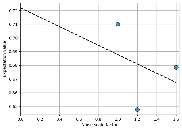
The plot shows the noise-amplified expectation values at each scale factor (data points) and the linear fit extrapolated to the zero-noise limit (zero on the x-axis).
Attention
Due to randomness in the PEA sampling protocol, the PEA error is not always guaranteed to be smaller than the noisy error.