Digital dynamical decoupling (DDD) with Qiskit on GHZ Circuits#
In this notebook DDD is applied to improve the success rate of the computation on a real hardware backend.
A similar approach can be taken on a simulated backend, by setting the USE_REAL_HARDWARE option to False
and specifying a simulated backend from qiskit.providers.fake_provider, which includes a noise model that approximates the noise of the
real device.
In DDD, sequences of gates are applied to slack windows, i.e. single-qubit idle windows, in a quantum circuit. Applying such sequences can reduce the coupling between the qubits and the environment, mitigating the effects of noise. While the DDD module includes some built-in sequences, the user may choose to define others best suited to their application. For more information on DDD, see the section DDD section of the user guide.
Setup#
We begin by importing the relevant modules and libraries that we will require for the rest of this tutorial.
from typing import List, Callable
import numpy as np
from matplotlib import pyplot as plt

import qiskit
from qiskit_ibm_provider import IBMProvider

from mitiq.interface.mitiq_qiskit import to_qiskit
from mitiq import ddd, QPROGRAM
from mitiq.ddd import insert_ddd_sequences
Define DDD rules#
We now use Mitiq’s DDD rule, i. e., a function that generates DDD sequences of different length.
In this example, we test the performance of repeated I (default built into get_circuit below) and repeated IXIX, repeated XX, and XX sequences from Mitiq.
import cirq

def rep_ixix_rule(window_length: int) -> Callable[[int], QPROGRAM]:
    return ddd.rules.repeated_rule(
        window_length, [cirq.I, cirq.X, cirq.I, cirq.X]
    )

def rep_xx_rule(window_length: int) -> Callable[[int], QPROGRAM]:
    return ddd.rules.repeated_rule(window_length, [cirq.X, cirq.X])

# Set DDD sequences to test.
rules = [rep_ixix_rule, rep_xx_rule, ddd.rules.xx]

# Test the sequence insertion
for rule in rules:
    print(rule(10))
0: ───I───I───X───I───X───I───X───I───X───I───
0: ───X───X───X───X───X───X───X───X───X───X───
0: ───I───I───I───X───I───I───X───I───I───I───
Set parameters for the experiment#
# Total number of shots to use.
shots = 10000

# Qubits to use on the experiment.
num_qubits = 2

# Test at multiple depths.
depths = [10, 30, 50, 100]
Define the circuit#
We use Greenberger-Horne-Zeilinger (GHZ) circuits to benchmark the performance of the device. GHZ circuits are designed such that only two bitstrings \(|00...0 \rangle\) and \(|11...1 \rangle\) should be sampled, with \(P_0 = P_1 = 0.5\). As noted in Mooney et al. (2021) [71], when GHZ circuits are run on a device, any other measured bitstrings are due to noise. In this example the GHZ sequence is applied first, followed by a long idle window of identity gates and finally the inverse of the GHZ sequence. Therefore \(P_0 = 1\), and the frequency of the \(|0 \rangle\) bitstring is our target metric (in this example we only measure the first qubit).
def get_circuit(depth: int):
    """Returns a circuit composed of a GHZ sequence, idle windows,
    and finally an inverse GHZ sequence.

    Args:
        depth: The depth of the idle window in the circuit.
    """
    circuit = qiskit.QuantumCircuit(num_qubits, num_qubits)
    circuit.h(0)
    circuit.cx(0, 1)
    for _ in range(depth):
        circuit.i(0)
        circuit.i(1)
    circuit.cx(0, 1)
    circuit.h(0)
    circuit.measure(0, 0)
    return circuit
Test the circuit output for depth 4, unmitigated
ibm_circ = get_circuit(4)
print(ibm_circ)
     ┌───┐     ┌───┐┌───┐┌───┐┌───┐     ┌───┐┌─┐
q_0: ┤ H ├──■──┤ I ├┤ I ├┤ I ├┤ I ├──■──┤ H ├┤M├
     └───┘┌─┴─┐├───┤├───┤├───┤├───┤┌─┴─┐└───┘└╥┘
q_1: ─────┤ X ├┤ I ├┤ I ├┤ I ├┤ I ├┤ X ├──────╫─
          └───┘└───┘└───┘└───┘└───┘└───┘      ║
c: 2/═════════════════════════════════════════╩═
                                              0
/tmp/ipykernel_960/4014706987.py:12: DeprecationWarning: The method ``qiskit.circuit.quantumcircuit.QuantumCircuit.i()`` is deprecated as of qiskit 0.45.0. It will be removed no earlier than 3 months after the release date. Use QuantumCircuit.id as direct replacement.
  circuit.i(0)
/tmp/ipykernel_960/4014706987.py:13: DeprecationWarning: The method ``qiskit.circuit.quantumcircuit.QuantumCircuit.i()`` is deprecated as of qiskit 0.45.0. It will be removed no earlier than 3 months after the release date. Use QuantumCircuit.id as direct replacement.
  circuit.i(1)
Test the circuit output for depth 4, with IX sequences inserted
ixix_circ = insert_ddd_sequences(ibm_circ, rep_ixix_rule)
print(ixix_circ)
     ┌───┐     ┌───┐┌───┐┌───┐┌───┐     ┌───┐┌─┐
q_0: ┤ H ├──■──┤ I ├┤ X ├┤ I ├┤ X ├──■──┤ H ├┤M├
     └───┘┌─┴─┐├───┤├───┤├───┤├───┤┌─┴─┐└───┘└╥┘
q_1: ─────┤ X ├┤ I ├┤ X ├┤ I ├┤ X ├┤ X ├──────╫─
          └───┘└───┘└───┘└───┘└───┘└───┘      ║
c: 2/═════════════════════════════════════════╩═
                                              0
Define the executor#
Now that we have a circuit, we define the execute function which inputs a circuit and returns an expectation value -
here, the frequency of sampling the correct bitstring.
USE_REAL_HARDWARE = True
correct_bitstring=[0]
if USE_REAL_HARDWARE:
    provider = IBMProvider()
    backend = provider.get_backend("ibmq_lima")
else:
    from qiskit.providers.fake_provider import FakeLima as FakeLima
    backend = FakeLima()


def ibm_executor(
    circuit: qiskit.QuantumCircuit,
    shots: int,
    correct_bitstring: List[int],
    noisy: bool = True,
) -> float:
    """Executes the input circuit(s) and returns ⟨A⟩, where
    A = |correct_bitstring⟩⟨correct_bitstring| for each circuit.

    Args:
        circuit: Circuit to run.
        shots: Number of times to execute the circuit to compute the
            expectation value.
        correct_bitstring: Bitstring the circuit is expected to return, in the
            absence of noise.
    """
    if noisy:
        transpiled = qiskit.transpile(circuit, backend=backend, optimization_level=0)
        job = backend.run(transpiled, optimization_level=0, shots=shots)
    else:
        ideal_backand = qiskit.Aer.get_backend("qasm_simulator")
        job = ideal_backand.run(circuit, optimization_level=0, shots=shots)

    # Convert from raw measurement counts to the expectation value
    all_counts = job.result().get_counts()
    prob_zero = all_counts.get("".join(map(str, correct_bitstring)), 0.0) / shots
    return prob_zero
Run circuits with and without DDD#
data = []
for depth in depths:
    circuit = get_circuit(depth)
    noisy_value = ibm_executor(
            circuit, shots=shots, correct_bitstring=correct_bitstring
    )
    data.append((depth, "unmitigated", noisy_value))
    for rule in rules:
        ddd_circuit = insert_ddd_sequences(circuit, rule)
        ddd_value = ibm_executor(
            ddd_circuit, shots=shots, correct_bitstring=correct_bitstring
        )
        data.append((depth, rule.__name__, ddd_value))
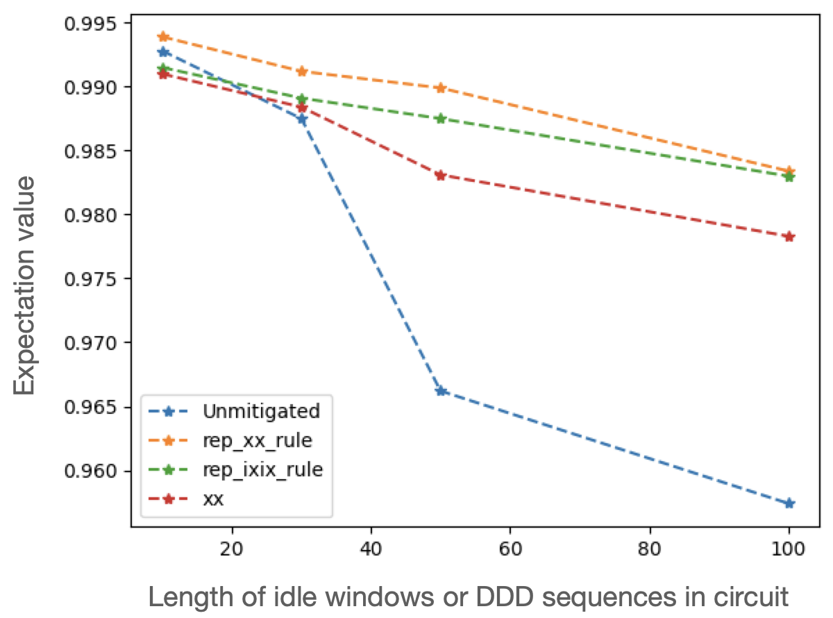
Now we can visualize the results.
# Plot unmitigated
x, y = [], []
for res in data:
    if res[1] == "unmitigated":
        x.append(res[0])
        y.append(res[2])
plt.plot(x, y, "--*", label="Unmitigated")

# Plot xx
x, y = [], []
for res in data:
    if res[1] == "rep_xx_rule":
        x.append(res[0])
        y.append(res[2])
plt.plot(x, y, "--*", label="rep_xx_rule")

# Plot ixix
x, y = [], []
for res in data:
    if res[1] == "rep_ixix_rule":
        x.append(res[0])
        y.append(res[2])
plt.plot(x, y, "--*", label="rep_ixix_rule")

# Plot xx
x, y = [], []
for res in data:
    if res[1] == "xx":
        x.append(res[0])
        y.append(res[2])
plt.plot(x, y, "--*", label="xx")


plt.legend()

Plot of the unmitigated and DDD-mitigated expectation values obtained from executing the corresponding circuits.#
We can see that DDD improves the expectation value at each circuit depth, and the repeated XX sequence is the best at mitigating the errors occurring during idle windows.
