Digital dynamical decoupling (DDD) with Mirror Circuits

In this notebook DDD is applied to improve the success rate of the computation. In DDD, sequences of gates are applied to slack windows, i.e. single-qubit idle windows, in a quantum circuit. Applying such sequences can reduce the coupling between the qubits and the environment, mitigating the effects of noise. For more information on DDD, see the section DDD section of the user guide.

Setup

We begin by importing the relevant modules and libraries that we will require for the rest of this tutorial.

import functools
from typing import List, Tuple

# Plotting imports.
import matplotlib.pyplot as plt

plt.rcParams.update({"font.family": "serif", "font.size": 15})
%matplotlib inline

# Third-party imports.
import cirq

import networkx as nx
import numpy as np

# Mitiq imports.
from mitiq import benchmarks, ddd

Define parameters

# Random seed for circuit generation.
seed = 1

# Total number of shots to use.
shots: int = 10000

# Qubits to use on the experiment.
qubits = [0, 1, 2]

# Average results over this many trials (circuit instances) at each depth.
trials = 3

# Clifford depths.
depths = [10, 20, 30]

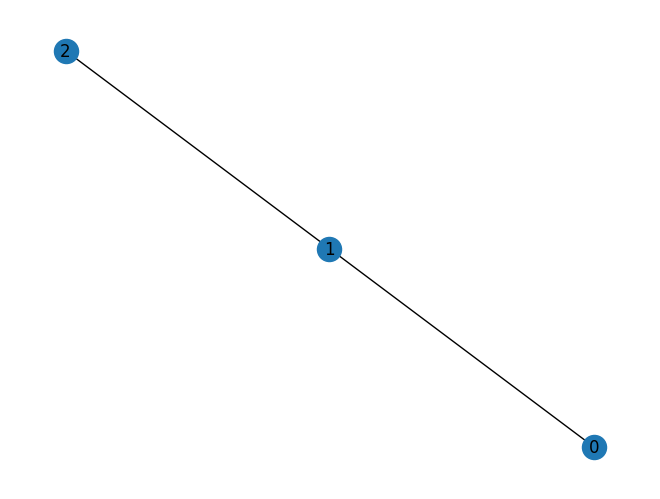
We also define a graph representation of our qubits and assume a line topology.

# Assume chain-like connectivity
topology = nx.Graph()
topology.add_edges_from([(0, 1), (1, 2)])
nx.draw(topology, with_labels=True)

# Add reversed edges to topology graph.
# This is important to represent CNOT gates with target and control reversed.
topology = nx.to_directed(topology)

Define the circuit

We use mirror circuits to benchmark the performance of the device. Mirror circuits, introduced in Proctor et al. (2021) [56], are designed such that only one bitstring should be sampled. When run on a device, any other measured bitstrings are due to noise. The frequency of the correct bitstring is our target metric.

Note

Mirror circuits build on Loschmidt echo circuits - i.e., circuits of the form \(U U^\dagger\) for some unitary \(U\). Loschmidt echo circuits are good benchmarks but have shortcomings - e.g., they are unable to detect coherent errors. Mirror circuits add new features to account for these shortcomings. For more background, see arXiv:2008.11294.

To define a mirror circuit, we need the device graph. We will use a subgraph of the device, and our first step is picking a subgraph with good qubits.

Generate mirror circuit

Now that we have the device graph, we can generate a mirror circuit and the bitstring it should sample as follows.

def get_circuit(depth: int, seed: int) -> Tuple[cirq.Circuit, List[int]]:
    circuit, correct_bitstring = benchmarks.generate_mirror_circuit(
        nlayers=depth,
        two_qubit_gate_prob=1.0,
        connectivity_graph=topology,
        two_qubit_gate_name="CNOT",
        seed=seed,
        return_type="cirq",
    )
    return circuit, correct_bitstring

Define the executor

Now that we have a circuit, we define the execute function which inputs a circuit and returns an expectation value - here, the frequency of sampling the correct bitstring.

Importantly, since DDD is designed to mitigate time-correlated (non-Markovian) noise, we simulate a particular noise model consisting of systematic \(R_Z\) rotations applied to each qubit after each moment. This corresponds to a dephasing noise which is strongly time-correlated and, therefore, likely to be mitigated by DDD.

def execute(
    circuit: cirq.Circuit,
    shots: int,
    correct_bitstring: List[int],
    is_noisy: bool = True,
) -> float:
    """Executes the input circuit(s) and returns ⟨A⟩, where
    A = |correct_bitstring⟩⟨correct_bitstring| for each circuit.
    """
    # This is useful to understand if DDD gates are inserted into the circuit.
    print(f"Executing circuit with {len(list(circuit.all_operations()))} gates.")
    if is_noisy:
        # Simulate systematic dephasing (coherent RZ) on each qubit for each moment.
        circuit_to_run = circuit.with_noise(cirq.rz(0.05))
    else:
        circuit_to_run = circuit.copy()

    circuit_to_run += cirq.measure(*sorted(circuit.all_qubits()), key="m")
    backend = cirq.DensityMatrixSimulator()

    result = backend.run(circuit_to_run, repetitions=shots)
    expval = result.measurements["m"].tolist().count(correct_bitstring) / shots
    return expval

Select the DDD sequences to be applied

We now import a DDD rule from Mitiq, i. e., a function that generates DDD sequences of different length. In this example, we opt for YY sequences (pairs of Pauli Y operations).

from mitiq import ddd

rule = ddd.rules.yy

Sample bitstrings from mirror circuits

true_values, noisy_values = [], []
ddd_values = []

noise_scaled_expectation_values = []

for depth in depths:
    print("Status: On depth", depth, end="\n\n")

    true_depth_values, noisy_depth_values, ddd_depth_values = [], [], []

    for trial in range(trials):
        # Local seed is calculated in this way to ensure that we don't get repeated values in loop.
        local_seed = 10**6 * depth + 10**3 * seed + trial

        circuit, correct_bitstring = get_circuit(depth, local_seed)

        true_value = execute(circuit, shots, correct_bitstring, is_noisy=False)
        noisy_value = execute(circuit, shots, correct_bitstring, is_noisy=True)

        noisy_executor = functools.partial(
            execute,
            shots=shots,
            correct_bitstring=correct_bitstring,
        )

        ddd_value = ddd.execute_with_ddd(
            circuit,
            noisy_executor,
            rule=rule,
        )

        ddd_depth_values.append(ddd_value)

        true_depth_values.append(true_value)
        noisy_depth_values.append(noisy_value)

    true_values.append(true_depth_values)
    noisy_values.append(noisy_depth_values)
    ddd_values.append(ddd_depth_values)

Status: On depth 10

Executing circuit with 137 gates.
Executing circuit with 137 gates.
Executing circuit with 157 gates.

Executing circuit with 145 gates.
Executing circuit with 145 gates.
Executing circuit with 180 gates.

Executing circuit with 147 gates.

Executing circuit with 147 gates.
Executing circuit with 178 gates.
Status: On depth 20

Executing circuit with 261 gates.
Executing circuit with 261 gates.

Executing circuit with 303 gates.
Executing circuit with 261 gates.

Executing circuit with 261 gates.
Executing circuit with 308 gates.

Executing circuit with 261 gates.
Executing circuit with 261 gates.

Executing circuit with 317 gates.
Status: On depth 30

Executing circuit with 383 gates.

Executing circuit with 383 gates.

Executing circuit with 447 gates.

Executing circuit with 375 gates.
Executing circuit with 375 gates.

Executing circuit with 420 gates.

Executing circuit with 381 gates.
Executing circuit with 381 gates.

Executing circuit with 449 gates.

Now we can visualize the results.

avg_true_values = np.average(true_values, axis=1)
avg_noisy_values = np.average(noisy_values, axis=1)

std_true_values = np.std(true_values, axis=1, ddof=1)
std_noisy_values = np.std(noisy_values, axis=1, ddof=1)

avg_ddd_values = np.average(ddd_values, axis=1)
std_ddd_values = np.std(ddd_values, axis=1, ddof=1)

plt.figure(figsize=(9, 5))

plt.plot(depths, avg_true_values, "--", label="True", lw=2)
eb = plt.errorbar(depths, avg_noisy_values, yerr=std_noisy_values, label="Raw", ls="-.")
eb[-1][0].set_linestyle("-.")
plt.errorbar(depths, avg_ddd_values, yerr=std_ddd_values, label="DDD")

plt.title(
    f"""Simulator with mirror circuits using ddd \nqubits {qubits}, {trials} trials."""
)
plt.xlabel("Depth")
plt.ylabel("Expectation value")
_ = plt.legend()

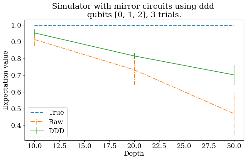
We can see that on average DDD slightly improves the expectation value. Note that the size of the error bars represents the standard deviation of the noisy values (for the “Raw” line) and the standard deviation of the DDD values (for the “DDD” line).