ZNE with Qiskit: Layerwise folding#
This tutorial shows an example of how to mitigate noise on IBMQ backends using layerwise folding in contrast with global folding.
One may ask why folding by layer is potentially beneficial to consider. One reason is that applying global folding will increase the length of the entire circuit while layerwise folding on a subset of only the noisiest layers will increase the circuit by a smaller factor.
If running a circuit on hardware is bottle-necked by the cost of running a long circuit, this technique could potentially be used to arrive at a better result (although not as good as global folding) but with less monetary cost.
More information on the layerwise folding technique can be found in Calderon et al. Quantum (2023) [7].
Setup#
import matplotlib.pyplot as plt
import numpy as np
import qiskit
from qiskit import QuantumCircuit
from qiskit_aer import QasmSimulator
from qiskit_aer.noise import NoiseModel
from qiskit_aer.noise.errors.standard_errors import depolarizing_error

from mitiq import zne
from mitiq.interface.mitiq_qiskit.qiskit_utils import sample_bitstrings
from mitiq.zne.scaling.layer_scaling import layer_folding

noise_model = NoiseModel()
noise_model.add_all_qubit_quantum_error(depolarizing_error(0.02, 1), ["x"])

backend = QasmSimulator(noise_model=noise_model)

shots = 10_000
Helper functions#
The following function will return a list of circuits where the ith element in
the list is a circuit with layer “i” folded num_folds number of times. This
will be useful when analyzing how much folding increases the noise on a given
layer.
def apply_num_folds_to_all_layers(
    circuit: QuantumCircuit, num_folds: int = 1
) -> list[QuantumCircuit]:
    """List of circuits where ``i``-th circuit is folded ``num_folds`` times."""
    return [
        layer_folding(
            circuit, [0] * i + [num_folds] + [0] * (len(circuit) - i)
        )
        for i in range(len(circuit))
    ]
For instance, consider the following circuit.
# Define a basic circuit for demonstration
circuit = QuantumCircuit(2, 1)
circuit.h(0)
circuit.cx(0, 1)
circuit.measure(0, 0)
print(circuit)
     ┌───┐     ┌─┐
q_0: ┤ H ├──■──┤M├
     └───┘┌─┴─┐└╥┘
q_1: ─────┤ X ├─╫─
          └───┘ ║
c: 1/═══════════╩═
                0
Let us invoke the apply_num_folds_to_all_layers function as follows.
folded_circuits = apply_num_folds_to_all_layers(circuit, num_folds=2)
Note that the first element of the list is the circuit with the first layer of the circuit folded twice.
print(folded_circuits[0])
     ┌───┐┌───┐┌───┐┌───┐┌───┐     ┌─┐
q_0: ┤ H ├┤ H ├┤ H ├┤ H ├┤ H ├──■──┤M├
     └───┘└───┘└───┘└───┘└───┘┌─┴─┐└╥┘
q_1: ─────────────────────────┤ X ├─╫─
                              └───┘ ║
c: 1/═══════════════════════════════╩═
                                    0
Similarly, the second element of the list is the circuit with the second layer folded.
print(folded_circuits[1])
     ┌───┐                         ┌─┐
q_0: ┤ H ├──■────■────■────■────■──┤M├
     └───┘┌─┴─┐┌─┴─┐┌─┴─┐┌─┴─┐┌─┴─┐└╥┘
q_1: ─────┤ X ├┤ X ├┤ X ├┤ X ├┤ X ├─╫─
          └───┘└───┘└───┘└───┘└───┘ ║
c: 1/═══════════════════════════════╩═
                                    0
Define circuit to analyze#
We will use the following circuit to analyze, but of course, you could use other circuits here as well.
circuit = QuantumCircuit(1, 1)
for _ in range(10):
    circuit.x(0)
circuit.measure(0, 0)
print(circuit)
     ┌───┐┌───┐┌───┐┌───┐┌───┐┌───┐┌───┐┌───┐┌───┐┌───┐┌─┐
  q: ┤ X ├┤ X ├┤ X ├┤ X ├┤ X ├┤ X ├┤ X ├┤ X ├┤ X ├┤ X ├┤M├
     └───┘└───┘└───┘└───┘└───┘└───┘└───┘└───┘└───┘└───┘└╥┘
c: 1/═══════════════════════════════════════════════════╩═
                                                        0
Total variational distance metric#
An \(i\)-inversion can be viewed as a local perturbation of the circuit. We want to define some measure by which we can determine how much such a perturbation affects the outcome.
Define the quantity:
as the probability distribution over measurement outcomes at the output of a circuit \(C\) where \(k \in B^n\) with \(B^n\) being the set of all \(n\)-length bit strings where \(\langle \langle k |\) is the vectorized POVM element that corresponds to measuring bit string \(k\).
The impact of applying an inversion is given by
where \(d\) is some distance measure. In Calderon et al. Quantum (2023) [7] the authors used the total variational distance (TVD) measure where
def tvd(
    circuit: QuantumCircuit, num_folds: int = 1, shots: int = 10_000
) -> dict[int, float]:
    """Compute the total variational distance (TVD) between ideal circuit and
    folded circuit(s)."""
    circuit_dist = sample_bitstrings(
        circuit, backend=backend, shots=shots
    ).prob_distribution()

    folded_circuits = apply_num_folds_to_all_layers(circuit, num_folds)

    distances: dict[int, float] = {}
    for i, folded_circuit in enumerate(folded_circuits):
        folded_circuit_dist = sample_bitstrings(
            folded_circuit,
            backend=backend,
            noise_model=noise_model,
            shots=shots,
        ).prob_distribution()

        res: float = 0.0
        for bitstring in circuit_dist.keys():
            res += np.abs(
                circuit_dist[bitstring] - folded_circuit_dist[bitstring]
            )
        distances[i] = res / 2

    return distances
Impact of single vs. multiple folding#
We can plot the impact of applying layer inversions to the circuit.
def plot_single_vs_multiple_folding(circuit: QuantumCircuit) -> None:
    """Plot how single vs. multiple folding impact the error at a given layer."""
    single_tvd = tvd(circuit, num_folds=1).values()
    multiple_tvd = tvd(circuit, num_folds=5).values()

    labels = [f"L{i}" for i in range(len(circuit))]
    x = np.arange(len(labels))  # the label locations
    width = 0.35  # the width of the bars

    fig, ax = plt.subplots()
    rects1 = ax.bar(x - width / 2, single_tvd, width, label="single")
    rects2 = ax.bar(x + width / 2, multiple_tvd, width, label="multiple")

    # Add some text for labels, title and custom x-axis tick labels, etc.
    ax.set_xlabel(r"$L_{G_i \theta_i}$")
    ax.set_ylabel(r"$\eta^{(i)}$")
    ax.set_title("Single vs. multiple folding")
    ax.set_xticks(x, labels, rotation=60)

    ax.legend()

    ax.bar_label(rects1, padding=3)
    ax.bar_label(rects2, padding=3)

    fig.tight_layout()

    plt.show()
plot_single_vs_multiple_folding(circuit)
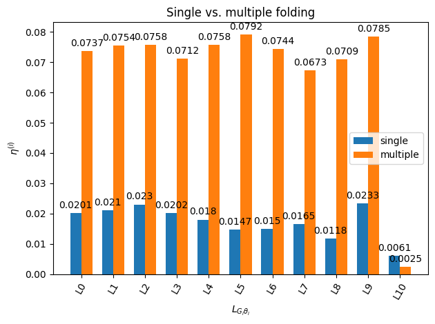
As can be seen, the amount of noise on each layer is increased if the number of folds on that layer are increased.
Executor#
Next, we define an executor function that will allow us to run our experiment
def executor(circuit: QuantumCircuit, shots: int = 10_000) -> float:
    """Returns the expectation value to be mitigated.

    Args:
        circuit: Circuit to run.
        shots: Number of times to execute the circuit to compute the expectation value.
    """
    # Transpile the circuit so it can be properly run
    exec_circuit = qiskit.transpile(
        circuit,
        backend=backend,
        basis_gates=noise_model.basis_gates if noise_model else None,
        optimization_level=0,  # Important to preserve folded gates.
    )
    # Run the circuit
    job = backend.run(exec_circuit, shots=shots)

    # Convert from raw measurement counts to the expectation value
    counts = job.result().get_counts()

    expectation_value = (
        0.0 if counts.get("0") is None else counts.get("0") / shots
    )
    return expectation_value
Global folding with linear extrapolation#
First, for comparison, we apply ZNE with global folding on the entire circuit. We then compare the mitigated result of applying ZNE with linear extrapolation against the unmitigated value.
unmitigated = executor(circuit)

linear_factory = zne.inference.LinearFactory(
    scale_factors=[1.0, 1.5, 2.0, 2.5, 3.0]
)
mitigated = zne.execute_with_zne(circuit, executor, factory=linear_factory)

print(f"Unmitigated result {unmitigated:.3f}")
print(f"Mitigated result {mitigated:.3f}")
/home/docs/checkouts/readthedocs.org/user_builds/mitiq/envs/stable/lib/python3.12/site-packages/qiskit/compiler/transpiler.py:269: UserWarning: Providing `coupling_map` and/or `basis_gates` along with `backend` is not recommended, as this will invalidate the backend's gate durations and error rates.
  pm = generate_preset_pass_manager(
Unmitigated result 0.912
Mitigated result 0.972
Layerwise folding with linear extrapolation#
For contrast, we apply layerwise folding on only the layer with the most noise and use linear extrapolation. As above, we compare the mitigated and unmitigated values.
# Calculate the TVDs of each layer in the circuit (with `num_folds=3`):
tvds = tvd(circuit, num_folds=3)

# Fold noisiest layer only.
layer_to_fold = max(tvds, key=tvds.get)
fold_layer_func = zne.scaling.get_layer_folding(layer_to_fold)

mitigated = zne.execute_with_zne(
    circuit, executor, scale_noise=fold_layer_func, factory=linear_factory
)
print(f"Mitigated (layerwise folding) result {mitigated:.3f}")
print(f"Unmitigated result {unmitigated:.3f}")
Mitigated (layerwise folding) result 0.919
Unmitigated result 0.912
/home/docs/checkouts/readthedocs.org/user_builds/mitiq/envs/stable/lib/python3.12/site-packages/qiskit/compiler/transpiler.py:269: UserWarning: Providing `coupling_map` and/or `basis_gates` along with `backend` is not recommended, as this will invalidate the backend's gate durations and error rates.
  pm = generate_preset_pass_manager(
Note
While doing layerwise folding on the noisiest layer will, on average, improve the mitigated value, it still will not eclipse the benefit of doing global folding.