Using ZNE and learning-based methods to mitigate the 1D transverse-longitudinal Ising model

In this tutorial, we employ ZNE, CDR, and VNCDR mitigation techniques to address errors in the simulation of the 1-D Transverse-Longitudinal Ising model using Mitiq. It is important to note that the results presented here are not original, but rather an attempt to reproduce some of the findings outlined in the paper available at [63].

One of the primary applications of quantum computers is simulating dynamics in many-body systems. This is particularly significant because as the system size increases, the number of parameters grows exponentially. As a result, classical computers struggle to efficiently simulate such dynamics. However, we are currently in the Noisy Intermediate-Scale Quantum (NISQ) era, which means we lack the necessary resources for fault-tolerant quantum computing. Nevertheless, Quantum Error Mitigation techniques have been developed to address noise using minimal qubit resources. These techniques harness the power of classical computers to handle and mitigate quantum noise. In quantum simulation, our main interest is usually finding the average value of an observable. However, NISQ hardware can only provide us with noisy results. In mitigation techniques, we combine these noisy results with the computational power of classical computers to combat the noise. In this tutorial, we specifically utilize Zero Noise Extrapolation (ZNE), Corrected Dynamical Reduction (CDR), and Variational Noise-Corrected Dynamical Reduction (VNCDR) techniques to mitigate errors in the simulation of a 1-D Ising Hamiltonian.

The Hamiltonian for the quantum one-dimensional Ising model, with both transverse and longitudinal fields, can be expressed as follows:

(1)\[\begin{equation} H = H_{ZZ} + H_Z + H_X, \end{equation}\]

(2)\[\begin{equation} H = -J\bigg[\sum_{i=1}^{L-1}Z_iZ_{i+1} + h_Z \sum_{i=1}^{L}Z_i + h_X\sum_{i=1}^L X_i\bigg]. \end{equation}\]

where J is an exchange coupling constant, which sets the microscopic energy scale and \(h_X\) and \(h_Z\) are the transverse and longitudinal relative field strengths, respectively. This model is integrable for \(h_Z = 0\) while for \(h_Z \neq 0\) it is only integrable in the continuum when \(h_X = 1\). The dynamics of this model is governed by the Schrödinger equation

(3)\[\begin{equation} \frac{d}{dt}\vert\Psi(t)\rangle = -i H\vert\Psi(t)\rangle, \end{equation}\]

which can formally be solved as

(4)\[\begin{equation} \vert\Psi(t + \Delta t)\rangle = e^{-i H\Delta t}\vert\Psi(t)\rangle = U(\Delta t)\vert\Psi(t)\rangle. \end{equation}\]

To simulate the dynamics using a gate sequence one performs a Trotter decomposition of this unitary operator, that is

(5)\[\begin{equation} U(\Delta t) \approx e^{-iH_{ZZ}\Delta t}e^{-iH_{Z}\Delta t}e^{-iH_{X}\Delta t}, \end{equation}\]

which is a product of different unitary operators. Finally, one can express each of these unitary operators as a gate sequence of single-qubit gates or two-qubit gates that are subsequently applied.

For the first step we import some packages.

import time

import cirq
import matplotlib.pyplot as plt
import numpy as np
from cirq.ops.common_channels import DepolarizingChannel

from mitiq import Observable, PauliString, cdr, zne
from mitiq.interface.mitiq_cirq import compute_density_matrix
from mitiq.observable import Observable, PauliString

import warnings
warnings.filterwarnings("ignore")

To start with coding, we define function “trotter_evolution_H” which is \(U(\Delta t)\)

"""
in the paper the example trotter circuit in fig. 12 is exp(iH*dt) instead of exp(-iH*dt).
To be consistent with their result I write the function for exp(iH*dt) too
"""


def trotter_evolution_H(
    L: int, h_z: float, h_x: float, Jdt: float
) -> cirq.Circuit:
    """Return the circuit that performs a time step.

    Args:
        L: Length of the Ising chain
        h_z: z interaction strength
        h_x: x interaction strength
        jdt: zz interaction strength time dt
    """
    # First define L qubits
    qubits = cirq.LineQubit.range(L)
    cq = cirq.Circuit()

    # Apply Rx gates:
    for ii in range(L):
        cq.append(cirq.rx(-2 * h_x * Jdt).on(qubits[ii]))

    # Apply Rz gates:
    for ii in range(L):
        cq.append(cirq.rz(-2 * h_z * Jdt).on(qubits[ii]))

    # We implement Rzz gate using two CNOT gates

    for ii in range(1, L - 1, 2):
        cq.append(cirq.CNOT(qubits[ii], qubits[ii + 1]))
        cq.append(cirq.rz(-2 * Jdt).on(qubits[ii + 1]))
        cq.append(cirq.CNOT(qubits[ii], qubits[ii + 1]))

    for ii in range(0, L - 1, 2):
        cq.append(cirq.CNOT(qubits[ii], qubits[ii + 1]))
        cq.append(cirq.rz(-2 * Jdt).on(qubits[ii + 1]))
        cq.append(cirq.CNOT(qubits[ii], qubits[ii + 1]))
    return cq

Instead of real hardware, we use a (Mitiq-wrapped) Cirq simulator to obtain the simulation results, and add depolarizing noise.

If you are interested, you can check out the tutorial here to find out how to do the same using IBM hardware https://mitiq.readthedocs.io/en/stable/examples/cirq-ibmq-backends.html

In addition, we define an exact simulator as we need to compare the exact and mitigated results.

def exact_simulator(circuit: cirq.Circuit) -> np.ndarray:
    return compute_density_matrix(circuit, noise_level=(0.0,))


def noisy_simulator(circuit: cirq.Circuit) -> np.ndarray:
    return compute_density_matrix(
        circuit, DepolarizingChannel, noise_level=(0.007,)
    )

We set the Hamiltonian parameters and simulate the Hamiltonian using the trotterization technique explained earlier. Then, we plot the average value of different observables. We begin by calculating the average value of \(Z_2\) when the initial state consists of all spins up.

L = 5
h_z = 0.9
h_x = 0.5
Jdt = 0.5
n_dt = 6  # number of time steps

# Create qubits
qubits = cirq.LineQubit.range(L)

# Create a circuit
test_circuit = cirq.Circuit()

# define the local observable Z_2
obs = Observable(PauliString("IIZ"))

# we create different lists variables for average value of Z_2 and its mitigated quantities
unmitigated_measurement = [1]
exact_measurement = [1]
mitigated_measurement_cdr = [1]
mitigated_measurement_vncdr = [1]
mitigated_measurement_zne = [1]

# repeat the trotter evolution n_dt times and compute compute the unmitigated, exact and mitigated quantities for each step using Mitiq
for ii in range(n_dt):
    test_circuit += trotter_evolution_H(L, h_z, h_x, Jdt)
    unmitigated_measurement.append(
        obs.expectation(test_circuit, noisy_simulator).real
    )
    exact_measurement.append(obs.expectation(test_circuit, exact_simulator))
    mitigated_measurement_vncdr.append(
        cdr.execute_with_cdr(
            test_circuit,
            noisy_simulator,
            observable=obs,
            simulator=exact_simulator,
            scale_factors=(1, 3),
        ).real
    )
    mitigated_measurement_cdr.append(
        cdr.execute_with_cdr(
            test_circuit,
            noisy_simulator,
            observable=obs,
            simulator=exact_simulator,
        ).real
    )
    mitigated_measurement_zne.append(
        zne.execute_with_zne(
            test_circuit,
            noisy_simulator,
            observable=obs,
        ).real
    )

    # this is to keep track of how fast the simulation is
    print(ii)

0

1

2

3

4

5

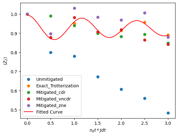
We plot all the exact, unmitigated, and different mitigated measurements to compare the results. As suggested in the original paper [63] , the evolution of the \(⟨Z_i(t)⟩\) is as follows

\( ⟨Z_i(t)⟩=a_1 e^{-a_2 t}\cos(a_3t)+a_4t+a_5 \)

we used the trotterized simulation results to estimate parametrs \(a_1, \dots ,a_5\).

import matplotlib.pyplot as plt
import numpy
from scipy.optimize import curve_fit


# Define the average value function
def sigma_z_t(x, a_1, a_2, a_3, a_4, a_5):
    return a_1 * numpy.exp(-a_2 * x) * numpy.cos(a_3 * x) + a_4 * x + a_5


# Generate some sample data
x_data = np.linspace(0, n_dt * Jdt, n_dt + 1)

# Fit the cosine function to the data
popt, pcov = curve_fit(sigma_z_t, x_data, exact_measurement)

# Extract the optimized parameters
a_1_opt, a_2_opt, a_3_opt, a_4_opt, a_5_opt = popt

# Generate the fitted curve
x_fit = np.linspace(0, n_dt * Jdt, 300)
y_fit = sigma_z_t(x_fit, *popt)

# Plot the  data sets and the fitted curve
plt.scatter(x_data, unmitigated_measurement, label="Unmitigated")
plt.scatter(x_data, exact_measurement, label="Exact_Trotterization")
plt.scatter(x_data, mitigated_measurement_cdr, label="Mitigated_cdr")
plt.scatter(x_data, mitigated_measurement_vncdr, label="Mitigated_vncdr")
plt.scatter(x_data, mitigated_measurement_zne, label="Mitigated_zne")
plt.plot(x_fit, y_fit, "r-", label="Fitted Curve")
plt.xlabel(r"$n_dt*Jdt$")
plt.ylabel(r"$\langle Z_2 \rangle$")
plt.legend()
plt.show()

We repeat the same thing using a different initial state. this time the initial state is \(\vert 00011⟩\)

# Create qubits
qubits = cirq.LineQubit.range(L)

# Create a circuit
test_circuit = cirq.Circuit()

# initialize the input state in|00011>
test_circuit.append(cirq.I(qubits[0]))
test_circuit.append(cirq.I(qubits[1]))
test_circuit.append(cirq.I(qubits[2]))
test_circuit.append(cirq.X(qubits[3]))
test_circuit.append(cirq.X(qubits[4]))

# define the local observable
obs = Observable(PauliString("IIZII"))

# repeat the trotter evolution n_dt times and compute compute the unmitigated, exact and mitigated quantities for each step
unmitigated_measurement = [1]
exact_measurement = [1]
mitigated_measurement_cdr = [1]
mitigated_measurement_vncdr = [1]
mitigated_measurement_zne = [1]
for ii in range(n_dt):
    test_circuit += trotter_evolution_H(L, h_z, h_x, Jdt)
    unmitigated_measurement.append(
        obs.expectation(test_circuit, noisy_simulator).real
    )
    exact_measurement.append(obs.expectation(test_circuit, exact_simulator))
    mitigated_measurement_cdr.append(
        cdr.execute_with_cdr(
            test_circuit,
            noisy_simulator,
            observable=obs,
            simulator=exact_simulator,
        ).real
    )
    mitigated_measurement_vncdr.append(
        cdr.execute_with_cdr(
            test_circuit,
            noisy_simulator,
            observable=obs,
            simulator=exact_simulator,
            scale_factors=(1, 3),
        ).real
    )
    mitigated_measurement_zne.append(
        zne.execute_with_zne(
            test_circuit,
            noisy_simulator,
            observable=obs,
        ).real
    )

    # this is to keep track of how fast the simulation is
    print(ii)

0

1

2

3

4

5

import numpy
from scipy.optimize import curve_fit
import matplotlib.pyplot as plt


# Define the cosine function
def func(x, a_1, a_2, a_3, a_4, a_5):
    return a_1 * numpy.exp(-a_2 * x) * numpy.cos(a_3 * x) + a_4 * x + a_5


# Generate some sample data
x_data = np.linspace(0, n_dt * Jdt, n_dt + 1)

# Fit the cosine function to the data
popt, pcov = curve_fit(func, x_data, exact_measurement)

# Extract the optimized parameters
a_1_opt, a_2_opt, a_3_opt, a_4_opt, a_5_opt = popt

# Generate the fitted curve
x_fit = np.linspace(0, n_dt * Jdt, 300)
y_fit = func(x_fit, *popt)

# Plot the original data and the fitted curve
plt.scatter(x_data, unmitigated_measurement, label="Unmitigated")
plt.scatter(x_data, exact_measurement, label="Exact_Trotterization")
plt.scatter(x_data, mitigated_measurement_cdr, label="Mitigated_cdr")
plt.scatter(x_data, mitigated_measurement_vncdr, label="Mitigated_vncdr")
plt.scatter(x_data, mitigated_measurement_zne, label="Mitigated_zne")
plt.plot(x_fit, y_fit, "r-", label="Fitted Curve")
plt.xlabel("n_dt * Jdt")
plt.ylabel("$<Z_2>$")
plt.legend()
plt.show()

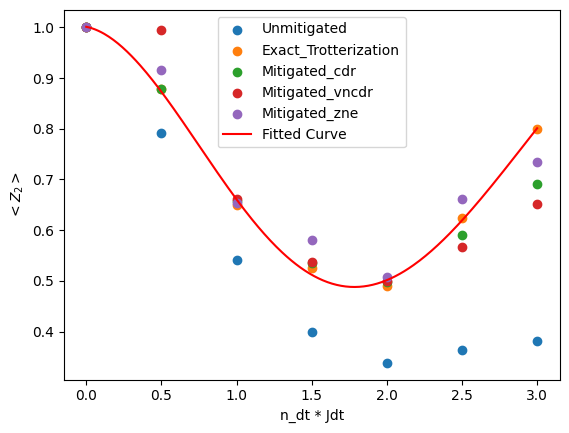
One can see that for both different initial states the mitigated results perform much better than the unmitigated results.

In order to show the temporal evolution of the position of fermions and mesons in this 1-D model, one should measure the probability distribution of kinks [63]

(6)\[\begin{equation} \Delta_i=\frac{1}{2} (I-Z_i Z_{i+1}). \end{equation}\]

We assess the effectiveness of various mitigation techniques in the simulation of operatore \(Δ_i\)

delta = [1] * 4

# define the \delta_i^zz observables
delta[0] = Observable(PauliString("ZZIII", -1 / 2), PauliString("I", 1 / 2))
delta[1] = Observable(PauliString("IZZII", -1 / 2), PauliString("I", 1 / 2))
delta[2] = Observable(PauliString("IIZZI", -1 / 2), PauliString("I", 1 / 2))
delta[3] = Observable(PauliString("IIIZZ", -1 / 2), PauliString("I", 1 / 2))

# Create qubits
qubits = cirq.LineQubit.range(L)

# Create a circuit
test_circuit = cirq.Circuit()

# initialize the input state in|00100>
test_circuit.append(cirq.I(qubits[0]))
test_circuit.append(cirq.I(qubits[1]))
test_circuit.append(cirq.X(qubits[2]))
test_circuit.append(cirq.I(qubits[3]))
test_circuit.append(cirq.I(qubits[4]))

# for each mitigation method we need a 4*n_dt matrix to save the results
unmitigated_measurement = [[1] * (n_dt) for _ in range(4)]
exact_measurement = [[1] * (n_dt) for _ in range(4)]
mitigated_measurement_cdr = [[1] * (n_dt) for _ in range(4)]
mitigated_measurement_vncdr = [[1] * (n_dt) for _ in range(4)]
mitigated_measurement_zne = [[1] * (n_dt) for _ in range(4)]

# repeat the trotter evolution n_dt times and compute compute the unmitigated, exact and mitigated quantities for each step
for ii in range(n_dt):
    for jj in range(4):
        unmitigated_measurement[jj][ii] = (
            delta[jj].expectation(test_circuit, noisy_simulator).real
        )
        exact_measurement[jj][ii] = delta[jj].expectation(
            test_circuit, exact_simulator
        )
        mitigated_measurement_cdr[jj][ii] = cdr.execute_with_cdr(
            test_circuit,
            noisy_simulator,
            observable=delta[jj],
            simulator=exact_simulator,
        ).real
        mitigated_measurement_vncdr[jj][ii] = cdr.execute_with_cdr(
            test_circuit,
            noisy_simulator,
            observable=delta[jj],
            simulator=exact_simulator,
            scale_factors=(1, 3),
        ).real
        mitigated_measurement_zne[jj][ii] = zne.execute_with_zne(
            test_circuit,
            noisy_simulator,
            observable=delta[jj],
        ).real
    test_circuit += trotter_evolution_H(L, h_z, h_x, Jdt)

    print(ii)

0

1

2

3

4

5

Then, we plot different simulations using color plots

# Plot exact_measurement using colors
plt.imshow(np.transpose(exact_measurement), cmap="viridis")

# Invert the y-axis
plt.gca().invert_yaxis()

# Add a title
plt.title("Exact Trotterization")

# Add x and y labels
plt.xlabel(r"$\Delta_i$")
plt.ylabel("n_dt")

# Add a colorbar for reference
plt.colorbar()

# Show the plot
plt.show()

# Plot unmitigated_measurement using colors
plt.imshow(np.transpose(unmitigated_measurement), cmap="viridis")

# Invert the y-axis
plt.gca().invert_yaxis()

# Add a title
plt.title("Unmitigated")

# Add x and y labels
plt.xlabel(r"$\Delta_i$")
plt.ylabel("n_dt")

# Add a colorbar for reference
plt.colorbar()

# Show the plot
plt.show()


# Plot mitigated_measurement_zne using colors
plt.imshow(np.transpose(mitigated_measurement_zne), cmap="viridis")

# Invert the y-axis
plt.gca().invert_yaxis()

# Add a title
plt.title("Mitigated ZNE")

# Add x and y labels
plt.xlabel(r"$\Delta_i$")
plt.ylabel("n_dt")

# Add a colorbar for reference
plt.colorbar()

# Show the plot
plt.show()


# Plot mitigated_measurement_cdr using colors
plt.imshow(np.transpose(mitigated_measurement_cdr), cmap="viridis")

# Invert the y-axis
plt.gca().invert_yaxis()

# Add a title
plt.title("Mitigated CDR")

# Add x and y labels
plt.xlabel(r"$\Delta_i$")
plt.ylabel("n_dt")

# Add a colorbar for reference
plt.colorbar()

# Show the plot
plt.show()

# Plot mitigated_measurement_vncdr using colors
plt.imshow(np.transpose(mitigated_measurement_vncdr), cmap="viridis")

# Invert the y-axis
plt.gca().invert_yaxis()

# Add a title
plt.title("Mitigated VNCDR")

# Add x and y labels
plt.xlabel(r"$\Delta_i$")
plt.ylabel("n_dt")

# Add a colorbar for reference
plt.colorbar()

# Show the plot
plt.show()

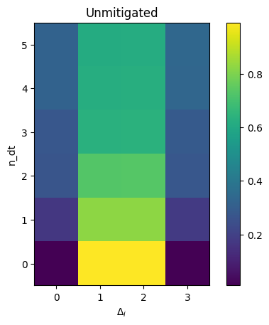
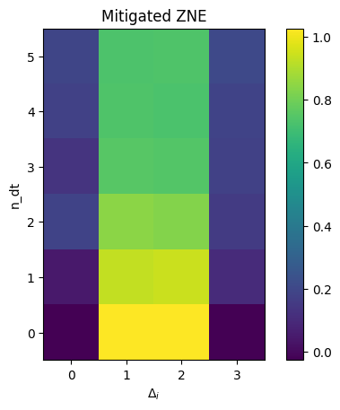
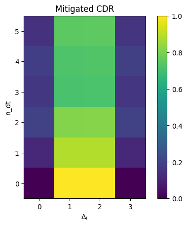
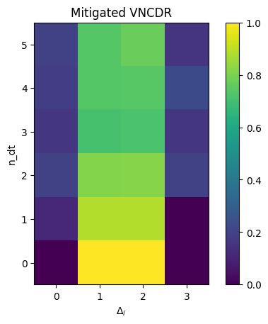
The plots are consist of different cells, and the color of each cell represents the value of \(\Delta_i\) at that particular time.

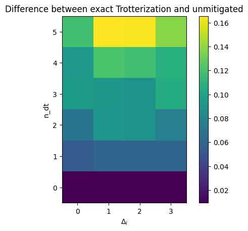
To enhance the visualization of the performance of various mitigation techniques, the absolute value of the difference between the exact measurement and different mitigation techniques is presented.

# Plot the difference between exact and unmitigated_measurement using colors
plt.imshow(
    np.abs(
        np.transpose(exact_measurement) - np.transpose(unmitigated_measurement)
    ),
    cmap="viridis",
)

# Invert the y-axis
plt.gca().invert_yaxis()

# Add a title
plt.title("Difference between exact Trotterization and unmitigated")

# Add x and y labels
plt.xlabel(r"$\Delta_i$")
plt.ylabel("n_dt")

# Add a colorbar for reference
plt.colorbar()

# Show the plot
plt.show()

# Plot the difference between exact and mitigated_measurement_zne using colors
plt.imshow(
    np.abs(
        np.transpose(exact_measurement)
        - np.transpose(mitigated_measurement_zne)
    ),
    cmap="viridis",
)

# Invert the y-axis
plt.gca().invert_yaxis()

# Add a title
plt.title("Difference between exact Trotterization and mitigated ZNE")

# Add x and y labels
plt.xlabel(r"$\Delta_i$")
plt.ylabel("n_dt")

# Add a colorbar for reference
plt.colorbar()

# Show the plot
plt.show()

# Plot the difference between exact and mitigated_measurement_cdr using colors
plt.imshow(
    np.abs(
        np.transpose(exact_measurement)
        - np.transpose(mitigated_measurement_cdr)
    ),
    cmap="viridis",
)

# Invert the y-axis
plt.gca().invert_yaxis()

# Add a title
plt.title("Difference between exact Trotterization and mitigated CDR")

# Add x and y labels
plt.xlabel(r"$\Delta_i$")
plt.ylabel("n_dt")

# Add a colorbar for reference
plt.colorbar()

# Show the plot
plt.show()

# Plot the difference between exact and mitigated_measurement_vncdr using colors
plt.imshow(
    np.abs(
        np.transpose(exact_measurement)
        - np.transpose(mitigated_measurement_vncdr)
    ),
    cmap="viridis",
)

# Invert the y-axis
plt.gca().invert_yaxis()

# Add a title
plt.title("Difference between exact Trotterization and mitigated VNCDR")

# Add x and y labels
plt.xlabel(r"$\Delta_i$")
plt.ylabel("n_dt")

# Add a colorbar for reference
plt.colorbar()

# Show the plot
plt.show()

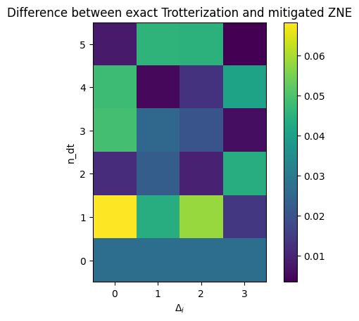
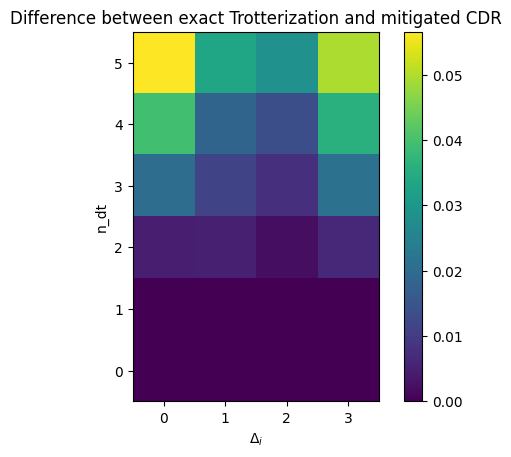
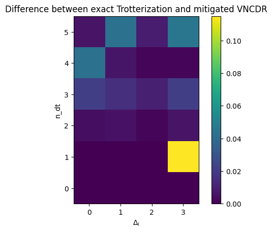
As one can see, the VNCDR method out performs the other methods and is much better than the unmitigated result.