ZNE on Stim backend with Cirq: Logical randomized benchmarking circuits#

This tutorial demonstrates a method of combining quantum error mitigation (QEM) and quantum error correction (QEC), with the goal of reducing the effective logical error rate of the computation. While QEM techniques such as zero noise extrapolation (ZNE) and probabilistic error cancellation are typically thought of as belonging to the NISQ regime, recently it has been shown that they can also benefit applications within the fault-tolerant regime [65, 66, 67]. In this example, we will apply ZNE with noise scaling by global unitary folding on logical randomized benchmarking (RB) circuits. This tutorial also introduces the use of Mitiq’s ZNE functions with Cirq as the frontend and the Stim stabilizer simulator as the backend.

Setup#

Since Stim is not a Mitiq-supported frontend, and the stimcirq library has a conversion utility for Cirq and Stim circuits, we will use Cirq as the frontend for this example.

import matplotlib as mpl
import numpy as np

import stim
import stimcirq
import cirq

import mitiq

In this example, we assume a physical error rate of 0.004 and a threshold of 0.009. Since the physical error rate is below the threshold, the computation is operating in the fault-tolerant regime.

n_qubits = 2
p_err = 0.004
p_th = 0.009
base_shots = 10**4
device_size = 1500

Randomized benchmarking is typically performed at the physical level, but it can be applied at the logical level as shown in Ref [68]. The modularity of logical RB circuits allows for parallelization of circuit executions, as permitted by the size of the device and number of physical qubits required for the logical circuit. To generate the RB circuits, we use a built-in Mitiq function, benchmarks.randomized_benchmarking.generate_rb_circuits(), where the n_cliffords argument refers to the number of Clifford groups in the circuit, and therefore scales the depth of the circuit. In this example the Clifford depth is 100, which would be around the limit of classical simulability if the operations in the circuit were instead non-Clifford.

trials = 10
n_cliffords = 100
cirq_circuits = mitiq.benchmarks.generate_rb_circuits(
    n_qubits, n_cliffords, trials
)

We also fill the idle windows of the circuit with identity gates, to which we will later append append \(X\) and \(Z\) errors, as each moment of the circuit corresponds to one correction cycle.

def fill_circuit_with_identities(circ):
    qubits = circ.all_qubits()
    return cirq.Circuit([
        m.expand_to(qubits) for m in circ
    ])

filled_circuits = []
for c in cirq_circuits:
    filled_circuit = fill_circuit_with_identities(c)
    filled_circuit.append(cirq.measure(filled_circuit.all_qubits()))
    filled_circuits.append(filled_circuit)

Noise model#

The noise is modeled as single-qubit \(X\) and \(Z\) errors, with probability \(p_L\) given by an empirical formula from Ref. [69]:

(1)#\[p_L\cong 0.03(\frac{p}{p_\mathrm{th}})^{(d+1)/2}\]

def calculate_logical_error_rate(p_err, p_th, distance):
    """Create sweepable Pauli noise model."""
    logical_err = 0.03 * (p_err / p_th) ** int((distance + 1) / 2)
    return logical_err

def add_noise_to_stim_circuit(circuit, p_err, p_th, d):
    noisy = stim.Circuit()
    l_err = calculate_logical_error_rate(p_err, p_th, d)
    for instruction in circuit:
        noisy.append(instruction)
        # append X and Z errors after every operation, ignoring timing ticks
        if instruction.name != "TICK":
            noisy.append(
                "X_ERROR",
                instruction.targets_copy(),
                l_err,
            )
            noisy.append(
                "Z_ERROR",
                instruction.targets_copy(),
                l_err,
            )
    return noisy

Execute circuits#

The Stim executor defined below accepts a Stim circuit, to which it applies the noise model, and then compiles and executes. For more information on Mitiq-compatible executors, see the Executors section of the Mitiq user guide.

def stim_executor(circuit, p_err, p_th, distance, shots):
    noisy_stim_circ = add_noise_to_stim_circuit(circuit, p_err, p_th, distance)
    sampler = noisy_stim_circ.compile_sampler()
    result = sampler.sample(shots=shots)
    counts = np.count_nonzero(
        [r[0].astype(int) + r[1].astype(int) for r in result]
    )
    return 1 - counts / shots

We will simulate the RB circuits at six different code distances and corresponding logical error rates. The distance of the error correcting code parameterizes the size of the physical data block per logical qubit and is directly related to the number of errors the code can correct.

code_distances = range(21, 9, -2)

Given a fixed (serial) sampling budget, here base_shots = 10,000, at code distances below the maximum available on the device, we can parallelize executions of each logical RB circuit and thereby take additional samples simultaneously. Note that we are not cutting the RB circuits but instead virtually splitting up the device to run the same logical RB circuit instance multiple times in parallel, with fewer qubits used for correction. The function scale_shots calculates how many total samples we can take, assuming lower code distance executions can be parallelized. Fixing a sampling budget across unmitigated and mitigated workflows provides a fair comparison of the results in terms of the resources required.

def scale_shots(
    num_device_qubits, scaled_distance, base_shots, n_qubits_circuit
):
    used_qubits = n_qubits_circuit * scaled_distance**2
    return base_shots * int(num_device_qubits / used_qubits)

To minimize execution time, we convert each trial circuit only once, outside of the execution loop.

noisy_results = np.zeros((trials, len(code_distances)))
stim_circuits = [
    stimcirq.cirq_circuit_to_stim_circuit(c) for c in filled_circuits
]

for i, code_distance in enumerate(code_distances):
    for s, stim_circuit in enumerate(stim_circuits):
        noisy_results[s, i] = stim_executor(
            stim_circuit,
            p_err,
            p_th,
            code_distance,
            scale_shots(device_size, code_distance, 4 * base_shots, n_qubits),
        )

Next we apply ZNE with the noise scaling method of global unitary folding and scale factors [1, 3, 5, 7], to each trial circuit and at each code distance simulated in the unmitigated case. Unlike other Mitiq examples, here the lower-level scaling and extrapolation functions are called explicitly. The circuits used here are deeper than those of other Mitiq examples and therefore take longer to fold and convert (sampling time is less of a concern with Stim), so we want to fold and convert the circuit as few times as possible.

scale_factors = [1, 3, 5, 7]
fac = mitiq.zne.PolyFactory(scale_factors=scale_factors, order=3)
scaling = mitiq.zne.scaling.folding.fold_global

scaled_stim_circuits = []
for c in filled_circuits:
    scaled_stim_circuit = []
    for s in scale_factors:
        scaled_circuit = mitiq.zne.scaling.fold_global(c, s)
        scaled_stim_circuit.append(
            stimcirq.cirq_circuit_to_stim_circuit(scaled_circuit)
        )
    scaled_stim_circuits.append(scaled_stim_circuit)

mitigated_results = np.zeros((trials, len(code_distances)))

for i, code_distance in enumerate(code_distances):
    for s, scaled_stim_circuit in enumerate(scaled_stim_circuits):
        fac.reset()
        for f, c in zip(scale_factors, scaled_stim_circuit):
            fac.push(
                {"scale_factor": f},
                stim_executor(
                    c,
                    p_err,
                    p_th,
                    code_distance,
                    scale_shots(
                        device_size, code_distance, base_shots, n_qubits
                    ),
                ),
            )
        mitigated_results[s, i] = fac.reduce()

Plot results#

Finally, plot the mean unmitigated and ZNE-mitigated expectation values, averaged over the trial circuits, at every code distance simulated. The error bars indicate the standard deviation.

mpl.pyplot.errorbar(
    code_distances,
    np.mean(mitigated_results, axis=0),
    yerr=np.std(mitigated_results, axis=0),
    label="Folding, m = 100",
)

mpl.pyplot.errorbar(
    code_distances,
    np.mean(noisy_results, axis=0),
    yerr=np.std(noisy_results, axis=0),
    ls="--",
    marker="o",
    label="Unmitigated, m = 100",
)

mpl.pyplot.plot(
    code_distances,
    np.ones((len(code_distances), 1)),
    ls=":",
    marker="*",
    label="Ideal",
    lw=2,
)

mpl.rc("font", family="Times New Roman")
mpl.pyplot.title(
    r"""Expectation value of $A=|00\rangle\langle00|$ from RB circuits acting on logical qubits""",
    fontsize=12,
)
mpl.pyplot.xticks(ticks = code_distances)

mpl.pyplot.xlabel(r"Maximum code distance, $d_{i,0}$")
mpl.pyplot.ylabel(r"Expectation value, $E$")

mpl.pyplot.legend()
mpl.pyplot.show()

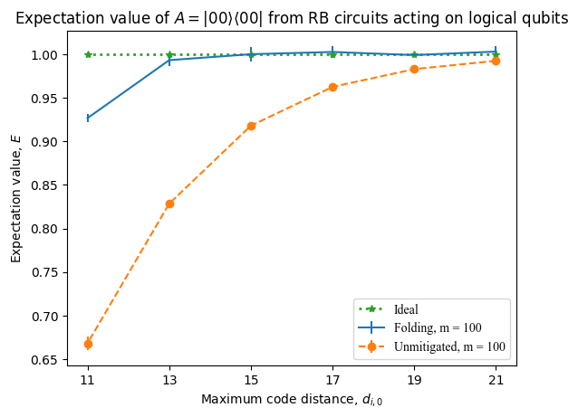
../_images/zne_stim.png — Plot of the unmitigated and ZNE-mitigated expectation values obtained from executing the logical RB circuits.#

We can see from the above plot that the ZNE-mitigated expectation values are closer to the ideal value of \(1.0\) at every code distance simulated. The effect is more pronounced at lower code distances, which correspond to a higher logical error rate, whereas by \(d = 21\) both the mitigated and unmitigated expectation values approach \(1.0\).

Note

Not all logical circuits can be folded, even at the circuit level. One alternative noise scaling method for logical qubits is scaling the code distance, which is referred to as distance-scaled ZNE or DS-ZNE [67].

Additional information on DS-ZNE#

Modeling the noise as in (1), assuming the computation is operating in the fault tolerant regime, we see that logical error rate decreases as code distance increases. We can therefore scale the noise level (here the logical error rate) by scaling the code distance and extrapolate back to the zero noise limit, obtaining an error-mitigated expectation value with a reduced effective logical error rate [67]. The DS-ZNE workflow implementation is contained in notebooks in the ds-zne folder of the unitaryfund/research repository.