Tags on this page: cirq shadows intermediate

Classical Shadows Protocol with Cirq

Corresponding to: Min Li (minl2@illinois.edu)

This notebook shows how to use classical shadows estimation with the Mitiq library, focused on local (Pauli) measurements. We demonstrate two common scenarios: state tomography and operator expectation value estimation. The method creates an approximate classical description of a quantum state using few measurements. The noise-robust extension of this protocol is demonstrated in the following notebook.

import cirq
import numpy as np
from mitiq.experimental.shadows.shadows import (
    classical_post_processing,
    shadow_quantum_processing,
)
from mitiq.experimental.shadows.shadows_utils import (
    fidelity,
    n_measurements_opts_expectation_bound,
    n_measurements_tomography_bound,
)
from mitiq import MeasurementResult
from mitiq.interface.mitiq_cirq.cirq_utils import (
    sample_bitstrings as cirq_sample_bitstrings,
)

/tmp/ipykernel_3055/3638331658.py:3: FutureWarning: mitiq.experimental.shadows is experimental and its API may change without notice in future releases. It is not covered by mitiq's semantic versioning guarantees.
  from mitiq.experimental.shadows.shadows import (

In an \(n\)-qubit system where \(\rho\) is an unknown quantum state in a \(2^n\)-dimensional Hilbert space, the classical shadows protocol extracts information about \(\rho\) through repeated randomized measurements.

Define a test circuit

def simple_test_circuit(
    angles: list[float], qubits: list[cirq.Qid]
) -> cirq.Circuit:
    circuit = cirq.Circuit()
    for i, qubit in enumerate(qubits):
        circuit.append(cirq.H(qubit))
        circuit.append(cirq.ry(angles[i])(qubit))
    for i in range(num_qubits - 1):
        circuit.append(cirq.CNOT(qubits[i], qubits[i + 1]))
    for i, qubit in enumerate(qubits):
        circuit.append(cirq.rz(angles[i + num_qubits])(qubit))
    return circuit


num_qubits = 4
qubits = cirq.LineQubit.range(num_qubits)
angles  = np.random.randn(2 * num_qubits)

test_circuit = simple_test_circuit(angles, qubits)
print(test_circuit)

0: ───H───Ry(-0.394π)───@───Rz(-0.199π)───────────────────────────────
                        │
1: ───H───Ry(-0.46π)────X───@─────────────Rz(-0.318π)─────────────────
                            │
2: ───H───Ry(-0.156π)───────X─────────────@─────────────Rz(-0.041π)───
                                          │
3: ───H───Ry(-0.44π)──────────────────────X─────────────Rz(0.188π)────

Sampling random Pauli measurements

The protocol samples a unitary \(U\) from a fixed ensemble \(\mathcal{U} \subseteq \mathsf{U}(2^n)\). The unitary is applied to the state, \(\rho \rightarrow U\rho U^\dagger\), after which the system is measured in the computational basis. A measurement outcome \(b \in \{0,1\}^n\) is obtained with probability

(1)\[\begin{equation} \Pr[b] = \langle b | U\rho U^\dagger | b \rangle. \end{equation}\]

For each shot we store a classical snapshot

(2)\[\begin{equation} U^\dagger |b\rangle\langle b| U, \end{equation}\]

which represents the measurement outcome rotated back into the original basis and forms the basic data structure used to reconstruct observables.

If the ensemble \(\mathcal{U}\) is chosen to be the local Clifford group \(\mathcal{C}_1^{\otimes n}\), this procedure is equivalent to performing a random Pauli measurement on each qubit: we randomly choose one of the three Pauli bases \(\{X, Y, Z\}\) per qubit.

Below, we define the cirq_executor to take a single shot and return the measurement result.

def cirq_executor(circuit: cirq.Circuit) -> MeasurementResult:
    return cirq_sample_bitstrings(
        circuit,
        noise_level=(0,),
        shots=1,
        sampler=cirq.Simulator(),
    )

The shadow_quantum_processing function encapsulates the quantum measurement process. It takes the circuit and the number of shots, and returns measurement outcomes as bitstrings (e.g., '01...0' represents \(|01 \cdots 0\rangle\)) together with the measured Pauli bases as strings (e.g., 'XY...Z' means \(X\) on qubit 0, \(Y\) on qubit 1, \(Z\) on the last qubit).

shadow_quantum_processing(test_circuit, cirq_executor, 2)

(['0000', '0110'], ['ZXXY', 'ZXYX'])

Snapshots and Classical Shadows

Each measurement produces a snapshot \(U^\dagger |b\rangle\langle b| U\) which depends on both \(U\) and the observed bitstring \(b\). Here, snapshot refers to a single measurement outcome transformed back to the original basis. Later, averaging these gives the classical shadow. A single snapshot is random, but the snapshots become more useful when we average over many snapshots We therefore consider the expectation over both the sampled unitary \(U \sim \mathcal{U}\) and the measurement outcome \(b\).

(3)\[\begin{equation} \mathbb{E}[U^\dagger |b\rangle\langle b| U] =: \mathcal{M}(\rho), \end{equation}\]

This defines a linear map \(\mathcal{M}\), which turns out to be a quantum channel. Further, if the ensemble is tomographically complete, then the map is also invertible! Applying its inverse yields an unbiased estimator of the state, called a classical shadow.

(4)\[\begin{equation} \hat{\rho}_b := \mathcal{M}^{-1}(U^\dagger |b\rangle \langle b| U) \end{equation}\]

The subscript \(b\) is a reminder that this reconstruction is dependent on the snapshot we recorded previously.

Random Pauli Measurements

For random Pauli measurements, the unitary factorizes as a tensor product over qubits (\(U = \bigotimes_{i = 1}^n C_i\) where \(C_i \in \mathcal{C}_1\)), so each snapshot also factorizes. In this case the reconstruction rule simplifies and can be applied independently to each qubit:

(5)\[\begin{equation} \hat{\rho} = \bigotimes_{i=1}^{n}\left(3 U_i^\dagger |b_i\rangle\langle b_i|U_i - \mathbb{I}\right),\qquad |b_i\rangle \in \{0,1\}. \end{equation}\]

This simple formula is what the implementation uses to convert measurement outcomes into classical shadows (classical_snapshot function). Repeating the measurement procedure \(N\) times produces a collection of independent classical shadows

(6)\[\begin{equation} S(\rho, N) = \left\{\hat{\rho}_1, \hat{\rho}_2, \ldots, \hat{\rho}_N\right\}. \end{equation}\]

These snapshots form the classical shadow dataset from which many properties of the quantum state can be estimated.

State Reconstruction from Classical Shadows

State Reconstruction

A classical shadow provides an unbiased estimator of the quantum state. Averaging many snapshots therefore yields an estimate of the density matrix.

(7)\[\begin{equation} \rho_\mathrm{shadow} = \mathbb{E}[\hat{\rho}]. \end{equation}\]

This averaging is implemented in shadow_state_reconstruction. In classical_post_processing, we pass state_reconstruction=True to apply the inverse channel to each snapshot and then average them.

# error rate of state reconstruction epsilon < 1
epsilon = 1
# minimum number of measurements required for error rate epsilon
num_measurements = n_measurements_tomography_bound(epsilon, num_qubits)

print(f"required measurements: {num_measurements}")
bitstrings, bases = shadow_quantum_processing(
    test_circuit, cirq_executor, num_measurements
)

required measurements: 8704

# get shadow reconstruction of the density matrix
output = classical_post_processing(
    (bitstrings, bases),
    state_reconstruction=True,
)
rho_shadow = output["reconstructed_state"]

# compute the ideal state vector described by the input circuit
state_vector = test_circuit.final_state_vector().reshape(-1, 1)
# compute the density matrix
rho_true = state_vector @ state_vector.conj().T

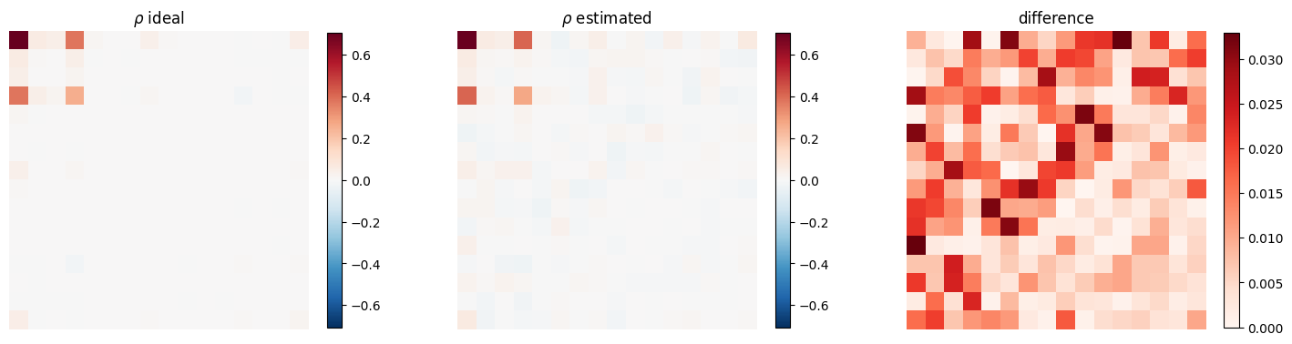
We can plot the element-wise difference between the reconstructed and true states as a heat map:

Show code cell source

Hide code cell source

import matplotlib.pyplot as plt

rho_shadow_real = np.real(rho_shadow)
rho_true_real = np.real(rho_true)
rho_diff = np.abs(rho_shadow_real - rho_true_real)

dm_abs_max = max(np.abs(rho_true_real).max(), np.abs(rho_shadow_real).max())

fig, axs = plt.subplots(1, 3, figsize=(18, 6))

for ax, data, title in zip(
    axs,
    [rho_true_real, rho_shadow_real, rho_diff],
    [r"$\rho$ ideal", r"$\rho$ estimated", "difference"],
):
    if title == "difference":
        im = ax.imshow(data, cmap="Reds", vmin=0, vmax=rho_diff.max())
    else:
        im = ax.imshow(data, cmap="RdBu_r", vmin=-dm_abs_max, vmax=dm_abs_max)
    fig.colorbar(im, ax=ax, orientation="vertical", shrink=0.7)
    ax.set_title(title)
    ax.axis("off")
plt.show()

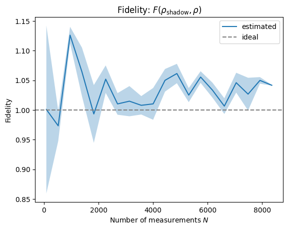
We also compute the fidelity as a function of the number of measurements to see how our state converges to the ideal.

Show code cell source

Hide code cell source

b_lists = np.array(bitstrings)
u_lists = np.array(bases)

n_measurement_list = np.arange(
    num_measurements // 100,
    num_measurements,
    num_measurements // 20,
)
n_runs = 3

fidelity_vals = np.zeros((len(n_measurement_list), n_runs))

for i, n_measurement in enumerate(n_measurement_list):
    # sample all runs at once: shape (n_runs, n_measurement)
    sample_idx = np.random.choice(len(b_lists), size=(n_runs, n_measurement), replace=True)
    for j, idx in enumerate(sample_idx):
        rho_shadow = classical_post_processing(
            shadow_outcomes=(b_lists[idx], u_lists[idx]),
            state_reconstruction=True,
        )["reconstructed_state"]
        fidelity_vals[i, j] = fidelity(rho_true, rho_shadow)

fidelity_mean = fidelity_vals.mean(axis=1)
fidelity_std = fidelity_vals.std(axis=1)

plt.figure()
plt.plot(n_measurement_list, fidelity_mean, label="estimated")
plt.fill_between(
    n_measurement_list,
    fidelity_mean - fidelity_std,
    fidelity_mean + fidelity_std,
    alpha=0.3,
)
plt.axhline(1.0, color="gray", linestyle="--", label="ideal")
plt.title(r"Fidelity: $F(\rho_\mathrm{shadow}, \rho)$")
plt.xlabel(r"Number of measurements $N$")
plt.ylabel("Fidelity")
plt.legend()
plt.show()

Estimating Expectation Values of Observables

The classical shadow \(\hat{\rho}\) allows us to estimate the expectation values of observables as well. For an observable \(O\):

(8)\[\begin{equation} \langle O \rangle = \mathrm{Tr}(O\hat{\rho}) \qquad \mathrm{Tr}(O\rho) \equiv \mathbb{E}[\langle O \rangle] \end{equation}\]

Averaging over \(N\) independent shadows gives an estimator:

(9)\[\begin{equation} \langle O\rangle(N) = \frac{1}{N}\sum_{i = 1}^N \mathrm{Tr}(O\hat{\rho}_i) \end{equation}\]

In other words, the classical shadow reproduces the expectation values of any linear function of the state in expectation.

As an example, we take our observables to be nearest-neighbor two-body interactions on a 1D lattice: \(O_i=P_i P_{i+1}\), where \(P_i\) is a Pauli operator on the \(i\)-th qubit.

from functools import partial

from mitiq import Observable, PauliString
from mitiq.interface import mitiq_cirq

list_of_paulistrings = (
    [PauliString("XX", support=(i, i + 1)) for i in range(num_qubits - 1)]
    + [PauliString("YY", support=(i, i + 1)) for i in range(num_qubits - 1)]
    + [PauliString("ZZ", support=(i, i + 1)) for i in range(num_qubits - 1)]
)

for observable in list_of_paulistrings:
    print(observable)

X(q(0))*X(q(1))
X(q(1))*X(q(2))
X(q(2))*X(q(3))
Y(q(0))*Y(q(1))
Y(q(1))*Y(q(2))
Y(q(2))*Y(q(3))
Z(q(0))*Z(q(1))
Z(q(1))*Z(q(2))
Z(q(2))*Z(q(3))

# compute exact expectation values ⟨O⟩ = Tr(O ρ)
expval_exact = []
for i, pauli_string in enumerate(list_of_paulistrings):
    obs = Observable(pauli_string)
    exp = obs.expectation(
        test_circuit,
        execute=partial(mitiq_cirq.compute_density_matrix, noise_level=(0.0,)),
    )
    expval_exact.append(exp)

For random Pauli measurements, only terms where the measured basis matches the observable contribute. The contribution is weighted according to the measurement outcome. This logic is handled automatically by Mitiq in classical_post_processing when state_reconstruction=False.

Acknowledgements

This project contains code adapted from PennyLane’s tutorial on Classical Shadows. We would like to acknowledge the original authors, PennyLane developers Brian Doolittle and Roeland Wiersema. The tutorial can be found at this link.