Tags on this page: shadows cirq intermediate

Robust Shadow Estimation with Mitiq

Corresponding to: Min Li (minl2@illinois.edu)

This notebook is a prototype of how to perform robust shadow estimation protocol with mitiq.

import cirq
import numpy as np
from typing import List
from mitiq.shadows.shadows import *
from mitiq.shadows.quantum_processing import *
from mitiq.shadows.classical_postprocessing import *
from mitiq.shadows.shadows_utils import *
from mitiq import MeasurementResult
from mitiq.interface.mitiq_cirq.cirq_utils import (
    sample_bitstrings as cirq_sample_bitstrings,
)

# set random seed
np.random.seed(666)

There are two options: Whether to run the quantum measurement or directly use the results from the previous run.

• If True, the measurement will be run again.

• If False, the results from the previous run will be used.

import zipfile, pickle, io, requests, os

run_quantum_processing = False
run_pauli_twirling_calibration = False

file_directory = "./resources"

if not run_quantum_processing:
    saved_data_name = "saved_data-rshadows"

    with zipfile.ZipFile(
        f"{file_directory}/rshadows-tutorial-{saved_data_name}.zip"
    ) as zf:
        saved_data = pickle.load(zf.open(f"{saved_data_name}.pkl"))

The robust shadow estimation[40] approach based on [39] exhibits noise resilience. The inherent randomization in the protocol simplifies the noise, transforming it into a Pauli noise channel that can be characterized relatively straightforwardly. Once the noisy channel \(\widehat{\mathcal{M}}\) is characterized, it is incorporated into the channel inversion \(\widehat{\mathcal{M}}^{-1}\), resulting in an unbiased state estimator. The sampling error in the determination of the Pauli channel contributes to the variance of this estimator.

1. Define Quantum Circuit and Executor

In this notebook, we’ll use the ground state of the Ising model with periodic boundary conditions as an example to study energy and two-point correlation function estimations. We’ll compare the performance of robust shadow estimation with the standard shadow protocol, taking into account the bit-flip or depolarization noise on the quantum channels.

The Hamiltonian of the Ising model is given by

(1)\[\begin{equation} H = -J\sum_{i=0}^{n-1} Z_i Z_{i+1} - g\sum_{i=1}^N X_i, \end{equation}\]

We focus on the case where \(J = g =1\). We use the ground state of such a system eight spins provided by

# import groud state of 1-D Ising model w/ periodic boundary condition
download_ising_circuits = True
num_qubits = 8
qubits: List[cirq.Qid] = cirq.LineQubit.range(num_qubits)

if download_ising_circuits:
    with open(f"{file_directory}/rshadows-tutorial-1D_Ising_g=1_{num_qubits}qubits.json", "rb") as file:
        circuit = cirq.read_json(json_text=file.read())
    g = 1

# or user can import from tensorflow_quantum
else:
    from tensorflow_quantum.datasets import tfi_chain

    qbs = cirq.GridQubit.rect(num_qubits, 1)
    circuits, labels, pauli_sums, addinfo = tfi_chain(qbs, "closed")
    lattice_idx = 40  # Critical point where g == 1
    g = addinfo[lattice_idx].g

    circuit = circuits[lattice_idx]
    qubit_map = {
        cirq.GridQubit(i, 0): cirq.LineQubit(i) for i in range(num_qubits)
    }

    circuit = circuit.transform_qubits(qubit_map=qubit_map)

Similar with the classical shadow protocol, we define the executor to perform the computational measurement for the circuit. Here, we use add single-qubit depolarizing noise after rotation gates but before the \(Z\)-basis measurement. As the noise is assumed to be gate independent, time invariant and Markovian, the noisy gate satisfies \(U_{\Lambda_U}(M_z)_{\Lambda_{\mathcal{M}_Z}}\equiv U\Lambda\mathcal{M}_Z\):

def cirq_executor(
    circuit: cirq.Circuit,
    noise_model_function=cirq.depolarize,
    noise_level=(0.2,),
    sampler=cirq.Simulator(),
) -> MeasurementResult:
    """
    This function returns the measurement outcomes of a circuit with noisy
    channel added right before measurement.
    Args:
        circuit: The circuit to execute.
    Returns:
        A one shot MeasurementResult object containing the measurement
        outcomes.
    """

    tmp_circuit = circuit.copy()
    qubits = sorted(list(tmp_circuit.all_qubits()))
    if noise_level[0] > 0:
        noisy_circuit = cirq.Circuit()
        operations = list(tmp_circuit)
        n_ops = len(operations)
        for i, op in enumerate(operations):
            if i == n_ops - 1:
                noisy_circuit.append(
                    cirq.Moment(
                        *noise_model_function(*noise_level).on_each(*qubits)
                    )
                )
            noisy_circuit.append(op)
        tmp_circuit = noisy_circuit
    # circuit.append(cirq.Moment(*noise_model_function(*noise_level).on_each(*qubits)))
    executor = cirq_sample_bitstrings(
        tmp_circuit,
        noise_model_function=None,
        noise_level=(0,),
        shots=1,
        sampler=sampler,
    )

    return executor

2. Pauli Twirling Calibration

2.1 PTM Representation

The PTM (Pauli Transfer Matrix) or Liouville representation provides a vector representation for all linear operators \(\mathcal{L}(\mathcal{H}_d)\) on an \(n\)-qubit Hilbert space \(\mathcal{H}_d\) (where \(d = 2^n\)). This representation uses the normalized Pauli operator basis \(\sigma_a=P_a/\sqrt{d}\), with \(P_a\) being the standard Pauli matrices.

from mitiq.utils import operator_ptm_vector_rep

operator_ptm_vector_rep(cirq.I._unitary_() / np.sqrt(2))

array([1.+0.j, 0.+0.j, 0.+0.j, 0.+0.j])

2.2 Pauli Twirling of Quantum Channel and Pauli Fidelity:

The classical shadow estimation involves Pauli twirling of a quantum channel represented by \(\mathcal{G} \subset U(d)\), with PTM representation \(\mathcal{U}\). This twirling allows direct computation of \(\widehat{\mathcal{M}}\) for the noisy channel \(\Lambda\):

(2)\[\begin{equation} \widehat{\mathcal{M}} = \mathbb{E}_{\mathcal{G}}[\mathcal{U}^\dagger\mathcal{M}_z\Lambda\mathcal{U}] \end{equation}\]

Local Clifford group projections are given by:

(3)\[\begin{equation} \Pi_{b_i}=\left\{ \begin{array}{ll} |\sigma_0\rangle\!\rangle\langle\!\langle\sigma_0|& b_i=0 \\ \mathbb{I}- |\sigma_0\rangle\!\rangle\langle\!\langle\sigma_0|& b_i = 1 \end{array}\right. \end{equation}\]

The Pauli fidelity for local Clifford group is:

(4)\[\begin{equation} \hat{f}^{(r)}_b = \prod_{i=1}^n \langle\!\langle b_i|\mathcal{U}_i|P_z^{b_i}\rangle\!\rangle \end{equation}\]

Final estimation is achieved using the median of means estimator. See get_single_shot_pauli_fidelity and mitiq.shadows.classical_postprocessing.get_pauli_fidelities for implementation.

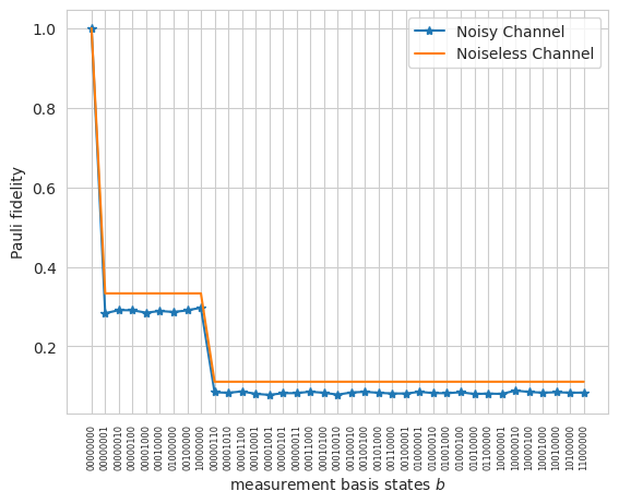
2.3 Noiseless Pauli Fidelity:

In the ideal noise-free scenario, Pauli fidelity is:

(5)\[\begin{equation} \hat{f}_{b}^{\mathrm{ideal}} = 3^{-|{b}|} \end{equation}\]

For noisy channels, the inverse channel \(\widehat{\mathcal{M}}^{-1}\) can be derived and used for robust shadow calibration, with differences attributed to variations in Pauli fidelity.

from functools import partial

n_total_measurements_calibration = 20000
if run_quantum_processing:
    noisy_executor = partial(cirq_executor, noise_level=(0.1,))
    zero_state_shadow_output = shadow_quantum_processing(
        # zero circuit of 8 qubits
        circuit=cirq.Circuit(),
        num_total_measurements_shadow=n_total_measurements_calibration,
        executor=noisy_executor,
        qubits=qubits,
    )
else:
    zero_state_shadow_output = saved_data["shadow_outcomes_f_plot"]
f_est_results = pauli_twirling_calibrate(
    zero_state_shadow_outcomes=zero_state_shadow_output,
    k_calibration=5,
    locality=2,
)

# sort bitstrings (b_lists' string rep) by number of 1s
bitstrings = np.array(sorted(list(f_est_results.keys())))

# reorder f_est_results by number of '1' in bitstrings
counts = {bitstring: bitstring.count("1") for bitstring in bitstrings}
order = np.argsort(list(counts.values()))
reordered_bitstrings = bitstrings[order]

# solve for theoretical Pauli fidelities
f_theoretical = {}
bitstrings = list(f_est_results.keys())
for bitstring in bitstrings:
    n_ones = bitstring.count("1")
    f_val = 3 ** (-n_ones)
    f_theoretical[bitstring] = f_val

import matplotlib.pyplot as plt
import seaborn as sns

sns.set_style("whitegrid")
# plot estimated vs theoretical Pauli fidelities when no errors in quantum circuit
plt.plot(
    [np.abs(f_est_results[b]) for b in reordered_bitstrings],
    "-*",
    label="Noisy Channel",
)
plt.plot(
    [f_theoretical[b] for b in reordered_bitstrings], label="Noiseless Channel"
)
plt.xlabel(r"measurement basis states $b$")
plt.xticks(
    range(len(reordered_bitstrings)),
    reordered_bitstrings,
    rotation="vertical",
    fontsize=6,
)

plt.ylabel("Pauli fidelity")
plt.legend();

3. Calibration of the operator expectation value estimation

The expectation value for a series of operators, denoted as \(\{O_\iota\}_{\iota\leq M}\), has a snapshot version of expectation value estimation by random Pauli measurement \(\widetilde{\mathcal{M}}=\bigotimes_{i}\widetilde{\mathcal{M}}_{P_i}\) and Pauli-twirling calibration \(\widehat{\mathcal{M}}^{-1}=\sum_{b\in\{0,1\}^n}f_b^{-1}\bigotimes_{i}\Pi_{b_i\in b}\), which is given by

(6)\[\begin{align} \hat{o}_\iota &= \langle\!\langle O_\iota|{\hat{\rho}}\rangle\!\rangle \simeq \langle\!\langle O_\iota|\widehat{\mathcal{M}}^{-1}\widetilde{\mathcal{M}}|\rho\rangle\!\rangle=\sum_{b^{(1)}\in\{0,1\}^{n}}f_{b^{(1)}}^{-1}\left(\bigotimes_{i=1}^n \langle\!\langle P_i|\Pi_{b_i^{(1)}}\widehat{\mathcal{M}}_{P_i}\right)|\rho\rangle\!\rangle\nonumber\\ &=\sum_{b^{(1)}\in\{0,1\}^{n}}f_{b^{(1)}}^{-1}\prod_{i=1}^n \langle\!\langle P_i|\Pi_{b^{(1)}_i}\bigg|U_i^{(2)\dagger}|b_i^{(2)}\rangle\langle b_i^{(2)}|U_i^{(2)}\bigg\rangle\!\bigg\rangle \end{align}\]

where in the last equality, \(\{P_i\}_{i\in n}\) represents Pauli operators, with \(P=\{I,X,Y,Z\}\). And as we did previously, we use the label \((1)\) as the subscript to distinguish the parameters of the calibration process from the parameters of the shadow estimation process, which is labelled by \((2)\). It is assumed that \(O_\iota\) are Pauli strings acting on \(supp(O_\iota)\) (\(|supp(O_\iota)|\leq n\)) sites of the system. It can be verified that the cross product over qubit sites within the summation of the final expression in the above equation is zero, except when all sites in \(supp(O_\iota)^c\) have \(\Pi_0\) acting on. Similarly, it can be verified that the cross product over qubit sites within the summation of the final expression in the above equation is zero, except when all sites in \(supp(O_\iota)\) have \(\Pi_1\) acting on, i.e.

(7)\[\begin{align} \Pi_i|I\rangle\!\rangle\equiv\delta_{i,0}|I\rangle\!\rangle,\qquad \Pi_{i}|P\rangle\!\rangle\equiv\delta_{i,1}|P\rangle\!\rangle,\qquad ~~~ \mathrm{for}~i\in\{0,1\};~P\;=\{X,\;Y,\;Z\}. \end{align}\]

Therefore, the final expression of the expectation value estimation can be simplified as

(8)\[\begin{align} \hat{o}_\iota = \left(\sum_{b^{(1)}\in\{0,1\}^{n}}f_{b^{(1)}}^{-1}\prod_{j\in supp(O_\iota)} \delta_{b_j^{(1)},1}\prod_{k\in supp(O_\iota)^c}\delta_{b_k^{(1)},0}\right)\prod_{i=1}^n \langle b_i^{(2)}|U_i^{(2)}P_i U_i^{(2)\dagger}|b_i^{(2)}\rangle \end{align}\]

Additionally, when \(P_i =X_i\) (r.e.s.p. \(Y_i,\;Z_i\)), \(U_i^{(2)}\) must correspond to \(X\) (r.e.s.p. \(Y,\;Z\))-basis measurement to yield a non-zero value, which is easy to check considered that the \(P\)-basis measurement channel has a PTM rep: \(\widetilde{\mathcal{M}}_{P}=\frac{1}{2}(|I\rangle\!\rangle\langle\!\langle I|+|P\rangle\!\rangle\langle\!\langle P|)\). Obviously, the only measurement that didn’t vanish by the operator’s \(i\)-th qubit component in PTM rep: \(P\rightarrow \langle\!\langle P|\), is the local \(P\)-basis measurement.

Next steps are identical to the classical protocol, where the statistical method of taking an average called “median of means” is used to achieve an acceptable failure probability of estimation. This needs \(R_2=N_2K_2\) snapshots, where we use the subscript “2” to denote the index of classical shadow protocol. Actually,

(9)\[\begin{align} \hat{o}_\iota(N_2,K_2):=\mathrm{median}\{\hat{o}_\iota^{(1)},\cdots,\hat{o}_\iota^{(K_2)}\}~~\mathrm{where}~~\hat{o}_\iota^{(j)}=N_2^{-1}\sum_{k=N_2(j-1)+1}^{N_2j}\mathrm{Tr}(O_\iota\hat{\rho}_k),\qquad \forall~1\leq j\leq K_2, \end{align}\]

where we have \(K_2\) estimators each of which is the average of \(N_2\) single-round estimators \(\hat{o}_i^{(j)}\), and take the median of these \(K_2\) estimators as our final estimator \(\hat{o}_\iota(N_2,K_2)\). We can calculate the median of means of each irreducible representations with projection \(\Pi_b=\bigotimes_{i=1}^n\Pi_{b_i}\),

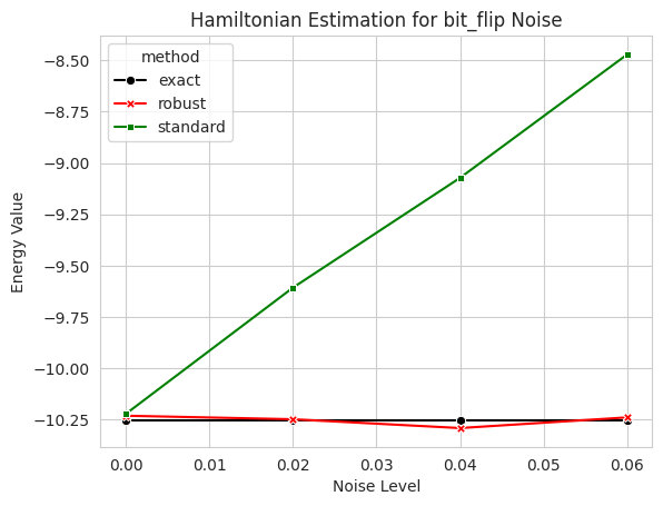
3.1 Ground State Energy Estimation of Ising model with the RSHADOWS algorithm

In this section, we will use the robust shadows estimation algorithm to estimate the ground state energy of the Ising model. We will use the compare_shadow_methods function to compare the performance of the robust shadows estimation algorithm and the classical shadows estimation algorithm. The compare_shadow_methods function takes the following parameters:

def compare_shadow_methods(
    circuit,
    observables,
    n_measurements_calibration,
    k_calibration,
    n_measurement_shadow,
    k_shadows,
    locality,
    noisy_executor,
    run_quantum_processing,
    shadow_measurement_result=None,
    zero_state_shadow_output=None,
):
    if run_quantum_processing:
        zero_state_shadow_output = shadow_quantum_processing(
            circuit=cirq.Circuit(),
            num_total_measurements_shadow=n_measurements_calibration,
            executor=noisy_executor,
            qubits=qubits,
        )
        shadow_measurement_result = shadow_quantum_processing(
            circuit,
            num_total_measurements_shadow=n_measurement_shadow,
            executor=noisy_executor,
        )
    else:
        assert shadow_measurement_result is not None
        assert zero_state_shadow_output is not None
        
    file_zsso = zero_state_shadow_output[1][0]
    file_k_cal = k_calibration
    file_locality = locality
    file_name = f"rshadows-tutorial-{file_zsso}-{file_k_cal}-{file_locality}"
    
    if not run_pauli_twirling_calibration and os.path.exists(f"{file_directory}/{file_name}.pkl"):
         # use the file
         with open(f"{file_directory}/{file_name}.pkl", "rb") as file:
             f_est = pickle.load(file)
    else:
        f_est = pauli_twirling_calibrate(
            zero_state_shadow_outcomes=zero_state_shadow_output,
            k_calibration=k_calibration,
            locality=locality,
        )
        
    output_shadow = classical_post_processing(
        shadow_outcomes=shadow_measurement_result,
        observables=observables,
        k_shadows=k_shadows,
    )

    output_shadow_cal = classical_post_processing(
        shadow_outcomes=shadow_measurement_result,
        calibration_results=f_est,
        observables=observables,
        k_shadows=k_shadows,
    )

    return {"standard": output_shadow, "robust": output_shadow_cal}

We use the groud state of 1-D Ising model with periodic boundary condition, with \(J= h=1\) for a Ising model with 8 spins as an example. The Hamiltonian is given by

# define obersevables lists as Ising model Hamiltonian
from mitiq import PauliString

ising_hamiltonian = [
    PauliString("X", support=(i,), coeff=-g) for i in range(num_qubits)
] + [
    PauliString("ZZ", support=(i, (i + 1) % num_qubits), coeff=-1)
    for i in range(num_qubits)
]

Calculate the exact expectation values of the Pauli operators for the above state:

state_vector = circuit.final_state_vector()
expval_exact = []
for i, pauli_string in enumerate(ising_hamiltonian):
    exp = pauli_string._pauli.expectation_from_state_vector(
        state_vector, qubit_map={q: i for i, q in enumerate(qubits)}
    )
    expval_exact.append(exp.real)

We use bit_flip channel as an example to show how to use the robust shadow estimation (RSE) in Mitiq. The bit_flip channel is a common noise model in quantum computing. It is a Pauli channel that flips the state of a qubit with probability \(p\).

noise_levels = np.linspace(0, 0.06, 4)
# if noise_model is None, then the noise model is depolarizing noise
noise_model = "bit_flip"

standard_results = []
robust_results = []
noise_model_fn = getattr(cirq, noise_model)
for noise_level in noise_levels:
    noisy_executor = partial(
        cirq_executor,
        noise_level=(noise_level,),
        noise_model_function=cirq.bit_flip,
    )

    experiment_name = f"{num_qubits}qubits_{noise_model}_{noise_level}"
    if run_quantum_processing:
        shadow_measurement_result, zero_state_shadow_output = None, None
    else:
        shadow_measurement_result = saved_data[experiment_name][
            "shadow_outcomes"
        ]
        zero_state_shadow_output = saved_data[experiment_name][
            "zero_shadow_outcomes"
        ]

    est_values = compare_shadow_methods(
        circuit=circuit,
        observables=ising_hamiltonian,
        n_measurements_calibration=60000,
        n_measurement_shadow=60000,
        k_shadows=6,
        locality=3,
        noisy_executor=noisy_executor,
        k_calibration=10,
        run_quantum_processing=False,
        shadow_measurement_result=shadow_measurement_result,
        zero_state_shadow_output=zero_state_shadow_output,
    )
    standard_results.append(est_values["standard"])
    robust_results.append(est_values["robust"])

import pandas as pd

df_energy = pd.DataFrame(
    columns=["noise_level", "method", "observable", "value"]
)
for i, noise_level in enumerate(noise_levels):
    est_values = {}
    est_values["standard"] = list(standard_results[i].values())
    est_values["robust"] = list(robust_results[i].values())
    # for j in range(len(standard_est_values)):
    df_energy = pd.concat(
        [
            df_energy,
            pd.DataFrame(
                {
                    "noise_level": noise_level,
                    "method": "exact",
                    "observable": [str(ham) for ham in ising_hamiltonian],
                    "value": expval_exact,
                }
            ),
        ],
        ignore_index=True,
    )
    for method in ["standard", "robust"]:
        df_energy = pd.concat(
            [
                df_energy,
                pd.DataFrame(
                    {
                        "noise_level": noise_level,
                        "method": method,
                        "observable": [str(ham) for ham in ising_hamiltonian],
                        "value": est_values[method],
                    }
                ),
            ],
            ignore_index=True,
        )

/tmp/ipykernel_1713/4023201604.py:11: FutureWarning: The behavior of DataFrame concatenation with empty or all-NA entries is deprecated. In a future version, this will no longer exclude empty or all-NA columns when determining the result dtypes. To retain the old behavior, exclude the relevant entries before the concat operation.
  df_energy = pd.concat(

df_hamiltonian = df_energy.groupby(["noise_level", "method"]).sum()
df_hamiltonian = df_hamiltonian.reset_index()
noise_model = "bit_flip"

# Define a color palette
palette = {"exact": "black", "robust": "red", "standard": "green"}

plt.figure()
sns.lineplot(
    data=df_hamiltonian,
    x="noise_level",
    y="value",
    hue="method",
    palette=palette,  # Use the color palette defined above
    markers=True,
    style="method",
    dashes=False,
    errorbar=("ci", 95),
)
plt.title(f"Hamiltonian Estimation for {noise_model} Noise")
plt.xlabel("Noise Level")
plt.ylabel("Energy Value");

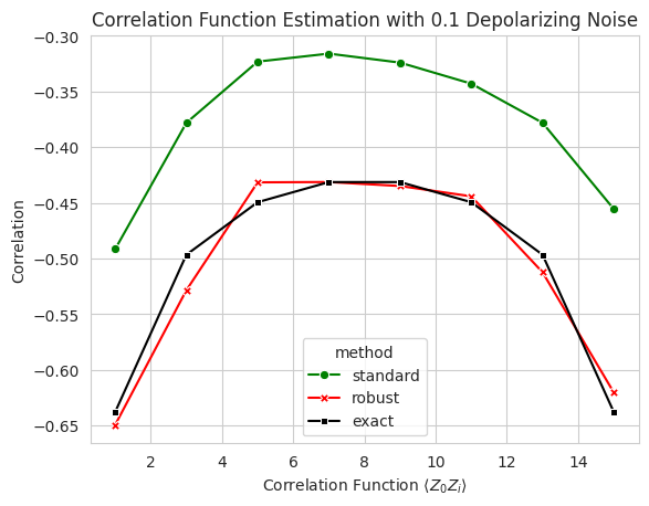
3.2 Two Point Correlation Function Estimation with RShadows

Let’s estimate two point correlation fuction: \(\langle Z_0 Z_i\rangle\) of a 16-spin 1D Ising model with transverse field on critical point ground state.

Import groud state of 1-D Ising model with periodic boundary condition

num_qubits = 16
qubits = cirq.LineQubit.range(num_qubits)
if download_ising_circuits:
    with open(f"{file_directory}/rshadows-tutorial-1D_Ising_g=1_{num_qubits}qubits.json", "rb") as file:
        circuit = cirq.read_json(json_text=file.read())
    g = 1
else:
    qbs = cirq.GridQubit.rect(num_qubits, 1)
    circuits, labels, pauli_sums, addinfo = tfi_chain(qbs, "closed")
    lattice_idx = 40  # Critical point where g == 1
    g = addinfo[lattice_idx].g
    circuit = circuits[lattice_idx]
    qubit_map = {
        cirq.GridQubit(i, 0): cirq.LineQubit(i) for i in range(num_qubits)
    }
    circuit = circuit.transform_qubits(qubit_map=qubit_map)

Define a list of observables as two point correlation functions between the first qubit and every other qubit \(\{\langle Z_0 Z_i\rangle\}_{0\leq i\leq n-1}\).

two_pt_correlation = [
    PauliString("ZZ", support=(0, i), coeff=-1) for i in range(1, num_qubits, 2)
]

Calculate the exact correlation function

expval_exact = []
state_vector = circuit.final_state_vector()
for i, pauli_string in enumerate(two_pt_correlation):
    exp = pauli_string._pauli.expectation_from_state_vector(
        state_vector, qubit_map={q: i for i, q in enumerate(qubits)}
    )
    expval_exact.append(exp.real)

with depolarizing noise set to \(0.1\), we compare the unmitigated and mitigated results:

noisy_executor = partial(cirq_executor, noise_level=(0.1,))
experiment_name = f"{num_qubits}qubits_depolarize_{noise_level}"
shadow_measurement_result = saved_data[experiment_name]["shadow_outcomes"]
zero_state_shadow_output = saved_data[experiment_name]["zero_shadow_outcomes"]

est_values = compare_shadow_methods(
    circuit=circuit,
    observables=two_pt_correlation,
    n_measurements_calibration=50000,
    n_measurement_shadow=50000,
    k_shadows=5,
    locality=2,
    noisy_executor=noisy_executor,
    k_calibration=5,
    run_quantum_processing=False,
    shadow_measurement_result=shadow_measurement_result,
    zero_state_shadow_output=zero_state_shadow_output,
)

df_corr = pd.DataFrame(
    columns=["method", "qubit_index", "observable", "value"]
)
qubit_idxes = [max(corr.support()) for corr in two_pt_correlation]
# for j in range(len(standard_est_values)):
for method in ["standard", "robust"]:
    df_corr = pd.concat(
        [
            df_corr,
            pd.DataFrame(
                {
                    "method": method,
                    "qubit_index": qubit_idxes,
                    "observable": [str(corr) for corr in two_pt_correlation],
                    "value": list(est_values[method].values()),
                }
            ),
        ],
        ignore_index=True,
    )
df_corr = pd.concat(
    [
        df_corr,
        pd.DataFrame(
            {
                "method": "exact",
                "qubit_index": qubit_idxes,
                "observable": [str(corr) for corr in two_pt_correlation],
                "value": expval_exact,
            }
        ),
    ],
    ignore_index=True,
)

/tmp/ipykernel_1713/2877321482.py:7: FutureWarning: The behavior of DataFrame concatenation with empty or all-NA entries is deprecated. In a future version, this will no longer exclude empty or all-NA columns when determining the result dtypes. To retain the old behavior, exclude the relevant entries before the concat operation.
  df_corr = pd.concat(

# Define a color palette
palette = {"exact": "black", "robust": "red", "standard": "green"}

plt.figure()
sns.lineplot(
    data=df_corr,
    x="qubit_index",
    y="value",
    hue="method",
    palette=palette,  # Use the color palette defined above
    markers=True,
    style="method",
    dashes=False,
    errorbar=("ci", 95),
)
plt.title("Correlation Function Estimation w/ 0.3 Depolarization Noise")
plt.xlabel(r"Correlation Function $\langle Z_0Z_i \rangle$")
plt.ylabel("Correlation");