Estimating the potential energy surface of molecular Hydrogen with ZNE and OpenFermion

In this example we apply zero-noise extrapolation (ZNE) to the estimation of the potential energy surface of molecular Hydrogen (\(\rm H_2\)). The variational algorithm used in this example is based on O’Malley et al. PRX (2016) [52].

With the appropriate settings (see code comments in the ZNE subsection), this notebook reproduces the results shown in Figure 4 of the Mitiq white paper.

Figure 1: Pictorial representation of the \(\rm H_2\) molecule. In this example, we variationally estimate the potential energy surface of the molecule as a function of the bond length \(R\).

from functools import partial
from typing import List
import matplotlib.pyplot as plt
import numpy as np
from scipy.optimize import brute
import cirq
import openfermion as of
from openfermionpyscf import generate_molecular_hamiltonian

from mitiq import PauliString, Observable, Executor, zne  # Zero-noise extrapolation module
from mitiq.interface.mitiq_cirq import compute_density_matrix

The Hamiltonian for \(\rm H_2\)

We can write down the Hamiltonian for \(\rm H_2\) in the following form [52]

(1)\[\begin{equation} H = g_0 I + g_1 Z_0 + g_2 Z_1 + g_3 Z_0 Z_1 + g_4 X_0 X_1 + g_5 Y_0 Y_1 \end{equation}\]

where \(g_i\) are numerical values that depend on the bond length \(R\). The above Hamiltonian:

1. Uses the minimal STO-6G basis,

2. Uses the Bravyi-Kitaev transform, and

3. Reduces resources (qubit number) by symmetry considerations (see [52] for more details).

Each coefficient \(g_i\) is a function of the bond length \(g_i = g_i(R)\). The exact parameters can be extracted from Appendix C of [52].

We can also calculate their values automatically using OpenFermion (an open source quantum chemistry package). To run the code of this example, the Python package openfermionpyscf must be installed in your system. This results in slightly modified hamiltonians of the form:

(2)\[\begin{equation} H = g_0 I + g_1 Z_0 + g_2 Z_1 + g_3 Z_0 Z_1 + g_4 X_0 X_1 \end{equation}\]

radii = [0.2 * i for i in range(1, 14)]

def qubit_operator_to_pauli_sum(qubit_op) -> List:
    """Converts the OpenFermion qubit operator to a list of mitiq Pauli Strings."""
    psum = []
    for ind_ops, coeff in qubit_op.terms.items():
        if ind_ops == tuple():
            psum.append(PauliString("I", coeff))
            continue
        term = ["I", "I"]
        for ind, op in ind_ops:
            term[ind] = op
        term = ''.join(term)
        psum.append(PauliString(term, coeff))
    return psum

def get_hamiltonian(bond_length) -> Observable:
    """Returns the hamiltonian for the H2 molecule at the given bond length. Uses the STO-6G basis set and the Bravyi-Kitaev
    transform to map fermionic operators to qubits. Results in a 2 qubit hamiltonian returned via a metriq.Observable."""
    geometry = [('H', (0., 0., 0.)), ('H', (0., 0., bond_length))]
    molecular_hamiltonian = generate_molecular_hamiltonian(geometry, basis='sto-6g', multiplicity=1, charge=0)
    fermionic_op = of.transforms.get_fermion_operator(molecular_hamiltonian)
    bk_op = of.transforms.symmetry_conserving_bravyi_kitaev(fermionic_op, active_orbitals=4, active_fermions=2)
    qubit_operator = qubit_operator_to_pauli_sum(bk_op)
    return Observable(*qubit_operator)

hamiltonians = [get_hamiltonian(i) for i in radii]
print(hamiltonians[0])

(2.1558922785125136+0j)*I + (1.0092918900420438+0j)*Z(q(0)) + (1.0092918900420438+0j)*Z(q(1)) + (0.013070708772819462+0j)*Z(q(0))*Z(q(1)) + (0.15813876498583737+0j)*X(q(0))*X(q(1))

Evaluating the energy landscape for a fixed \(R\)

We first define a function that returns single-parameter variational circuit. The ansatz is based on on Fig. 1 of [52].

def ansatz(theta: float) -> cirq.Circuit:
    """Returns the circuit associated to the input variational parameter."""
    qreg = cirq.LineQubit.range(2)
    return cirq.Circuit(
        cirq.ops.ry(np.pi / 2).on(qreg[0]),
        cirq.ops.rx(-np.pi / 2).on(qreg[1]),
        cirq.ops.CNOT.on(*qreg),
        cirq.ops.rz(theta).on(qreg[1]),
        cirq.ops.CNOT.on(*qreg),
        cirq.ops.ry(-np.pi / 2).on(qreg[0]),
        cirq.ops.rx(np.pi / 2).on(qreg[1]),
    )

Below we set a particular radius \(R\) and sweep the \(\theta\) parameter to evaluate the unmitigated energy landscape \(E(\theta, R)\) using different strengths \(p\) of depolarizing noise.

# Noise levels
pvals = (0.00, 0.02, 0.04)
# Variational parameters
thetas = np.linspace(0.0, 2.0 * np.pi, 10)

all_energies = []
for pval in pvals:
    energies = []
    for theta in thetas:
        results = hamiltonians[0].expectation(ansatz(theta), execute=partial(compute_density_matrix, noise_model_function=cirq.depolarize, noise_level=(pval,)))
        energies.append(np.real(results))
    all_energies.append(energies)

The unmitigated energy landscapes are now stored in the all_energies variable and will be visualized later.

Applying zero-noise extrapolation to estimate \(E(\theta, R)\)

We now use zero-noise extrapolation to error-mitigate the energy landscapes \(E(\theta, R)\) for a fixed value of \(R\) and for different levels of the noise.

# Set noise scaling method
scaling_function = zne.scaling.fold_global
# Set extrapolation method
fac = zne.inference.RichardsonFactory(scale_factors=[1, 3, 5])
# Set number of trials per expectation value
num_to_average = 1

# To reproduce the results of the Mitiq paper use the following settings
# scaling_function = zne.scaling.fold_gates_at_random
# pfac = zne.inference.PolyFactory(order=3,
#                           scale_factors=[1., 1.5, 2., 2.5, 3., 3.5, 4., 4.5, 5., 5.5, 6.])
# num_to_average = 5
# pvals = (0.00, 0.02, 0.04, 0.06)
# thetas = np.linspace(0.0, 2.0 * np.pi, 20)

all_mitigated = []
for p in pvals[1:]:
    mitigated = []
    for theta in thetas:
        # Define an executor function
        executor = Executor(partial(compute_density_matrix, noise_model_function=cirq.depolarize, noise_level=(p,)))
        # Run ZNE
        zne_value = zne.execute_with_zne(
            ansatz(theta),
            executor,
            hamiltonians[0],
            factory=fac,
            scale_noise=scaling_function,
            num_to_average=num_to_average,
        )
        mitigated.append(np.real(zne_value))
    all_mitigated.append(mitigated)

In the next figure we visualize the following results:

1. The ideal noiseless energy landscape \(E(\theta, R)\) corresponding to all_energies[0];

2. The noisy (unmitigated) energies all_energies;

3. The corresponding error-mitigated energies all_mitigated.

plt.rcParams.update({"font.family": "serif", "font.size": 14, "font.weight": "bold"})
plt.figure(figsize=(15, 5))
# Plot unmitigated results
plt.subplot(121)
plt.title("Unmitigated")
for i in range(len(all_energies)):
    plt.plot(
        thetas,
        all_energies[i],
        "--s",
        lw=3,
        markersize=10,
        markeredgecolor="black",
        alpha=0.7,
        label=f"$p = {pvals[i]}$",
    )
plt.xlabel(r"$\theta$")
plt.ylabel(r"$E(\theta)$")
plt.legend()
plt.subplot(122)
plt.title("Mitigated with ZNE")
# Plot noiseless results
plt.plot(
    thetas,
    all_energies[0],
    "--s",
    lw=3,
    markersize=10,
    markeredgecolor="black",
    alpha=0.7,
    label="$p = 0.0$",
)
# Plot error-mitigated results
for i in range(len(all_mitigated)):
    plt.plot(
        thetas,
        all_mitigated[i],
        "--o",
        lw=3,
        markersize=10,
        markeredgecolor="black",
        alpha=0.7,
        label=f"$p = {pvals[i + 1]}$",
    )
plt.xlabel(r"$\theta$")
plt.legend()
plt.tight_layout()

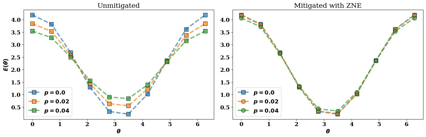
In the figure above, the error-mitigated energy landscapes (colored circles) are closer to the ideal noiseless limit (blue squares) when compared to the unmitigated values (colored squares).

Evaluating the potential energy surface \(V(R)\)

In the previous section we mitigated the energy landscape \(E(\theta, R)\) for a particular value of \(R\). Here instead we evaluate the potential energy surface, which can be defined as

\[V(R) = \min_\theta(E(\theta, R)). \]

We first evaluate \(V(R)\) without using error mitigation.

best_thetas = []
best_energies = []
for pval in pvals:
    print(f"\nStatus: p = {pval}")
    these_thetas = []
    these_energies = []
    for i in range(len(radii)):
        # Objective function to minimize
        def obj(theta):
            val = hamiltonians[i].expectation(
                ansatz(theta[0]),
                execute=partial(
                    compute_density_matrix,
                    noise_model_function=cirq.depolarize,
                    noise_level=(pval,),
                ),
            )
            return np.real(val)

        res = brute(
            obj, ranges=[(0, 2 * np.pi)], Ns=10, finish=None, full_output=True
        )
        these_thetas.append(res[0])
        these_energies.append(res[1])

    best_thetas.append(these_thetas)
    best_energies.append(these_energies)

Status: p = 0.0

Status: p = 0.02

Status: p = 0.04

The unmitigated potential energy surfaces are now stored in the best_energies variable and will be visualized later.

Applying zero-noise extrapolation to estimate \(V(R)\)

We use zero-noise extrapolation to error-mitigate the potential energy surface \(V(R)\).

best_mitigated_thetas = []
best_mitigated_energies = []
for pval in pvals[1:]:
    print(f"\nStatus: p = {pval}")
    these_thetas = []
    these_energies = []
    for i in range(len(radii)):

        def objective_function(theta):
            return np.real(zne.execute_with_zne(
                ansatz(theta),
                Executor(partial(compute_density_matrix, noise_model_function=cirq.depolarize, noise_level=(pval,))),
                hamiltonians[i],
                factory=fac,
                scale_noise=scaling_function,
                num_to_average=num_to_average,
            ))

        # Minimize energy with respect to "theta"
        res = brute(
            objective_function,
            ranges=[(0, 2 * np.pi)],
            Ns=10,
            finish=None,
            full_output=True,
        )
        these_thetas.append(res[0])
        these_energies.append(res[1])

    best_mitigated_thetas.append(these_thetas)
    best_mitigated_energies.append(these_energies)

Status: p = 0.02

Status: p = 0.04

In the next figure we visualize the following results:

1. The ideal noiseless potential energy surface \(V(R)\) corresponding to best_energies[0];

2. The noisy (unmitigated) potential energy surfaces best_energies;

3. The corresponding error-mitigated potential energy surfaces best_mitigated_energies.

plt.figure(figsize=(15, 5))
# Plot unmitigated results
plt.subplot(121)
plt.title("Unmitigated")
for pval, opt_energies in zip(pvals, best_energies):
    plt.plot(
        radii,
        opt_energies,
        "--s",
        lw=2,
        markersize=10,
        markeredgecolor="black",
        alpha=0.7,
        label=f"$p = {pval}$",
    )
plt.ylim(
    min([np.min(best_energies), np.min(best_mitigated_energies)]) - 0.1,
    max([np.max(best_energies), np.max(best_mitigated_energies)]) + 0.1,
)
plt.xlabel("Atomic distance (Angstroms)")
plt.ylabel("Energy (Hartree)")
plt.legend()
# Plot noiseless results
plt.subplot(122)
plt.title("Mitigated with ZNE")
plt.plot(
    radii,
    best_energies[0],
    "-s",
    lw=2,
    markersize=10,
    markeredgecolor="black",
    alpha=0.7,
    label=f"$p = 0.0$",
    zorder=1,
)
# Plot error-mitigated results
i = 0
for pval, opt_energies in zip(pvals[1:], best_mitigated_energies):
    i += 1
    plt.plot(
        radii,
        opt_energies,
        "-o",
        lw=2,
        markersize=10,
        markeredgecolor="black",
        alpha=0.7,
        label=f"$p = {pval}$",
        zorder=0,
    )
plt.ylim(
    min([np.min(best_energies), np.min(best_mitigated_energies)]) - 0.1,
    max([np.max(best_energies), np.max(best_mitigated_energies)]) + 0.1,
)

plt.xlabel("Atomic distance (Angstroms)")
plt.legend();

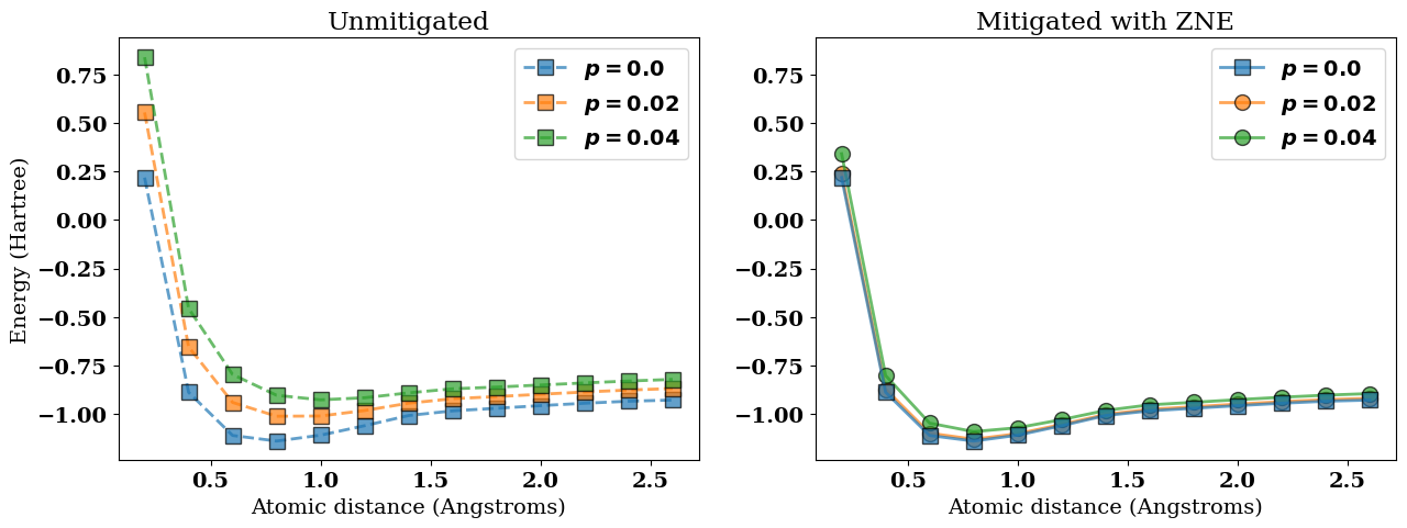
In the figure above, the error-mitigated potential energy surfaces (colored circles) are closer to the ideal noiseless limit (blue squares) when compared to the unmitigated results (colored squares).