Tags on this page: pt ddd rem zne advanced cirq

Advanced Error Mitigation Pipeline: Combining PT, DDD, REM, and ZNE#

Error mitigation techniques in quantum computing often address specific types of noise. In real quantum devices, multiple noise sources are present simultaneously, making it beneficial to combine different error mitigation strategies. This tutorial demonstrates how to build an advanced error mitigation pipeline by combining:

Pauli Twirling (PT): Converts coherent noise into stochastic Pauli noise.
Digital Dynamical Decoupling (DDD): Mitigates time-correlated noise by inserting decoupling sequences.
Readout Error Mitigation (REM): Corrects errors that occur during the measurement process.
Zero-Noise Extrapolation (ZNE): Suppresses generic gate noise by extrapolating results from circuits run at amplified noise levels back to the zero-noise limit.

We’ll implement a step-by-step approach, analyzing the impact of each technique individually. For DDD and ZNE, we will highlight the pattern of first constructing modified circuits, then executing them, and finally combining results. For REM, we’ll demonstrate generating the inverse confusion matrix, applying correction to measurement results, and computing mitigated expectation values.

Setup#

Let’s begin by importing the necessary libraries and modules.

import numpy as np
import matplotlib.pyplot as plt
import cirq
from functools import partial
import networkx as nx
from typing import List
import itertools

# Mitiq imports
import mitiq
from mitiq import MeasurementResult, Observable, PauliString
from mitiq.benchmarks.mirror_circuits import generate_mirror_circuit
from mitiq import pt, ddd, rem, zne
from mitiq.zne.inference import LinearFactory
from mitiq.zne.scaling import fold_global

Circuit and Observable#

For this tutorial, we’ll use a mirror circuit to benchmark our error mitigation techniques. Mirror circuits are designed to return to a known computational basis state after a sequence of randomized operations, making them excellent benchmarks for quantum error mitigation.

To ensure our observable correctly measures the fidelity with respect to the mirror circuit’s expected output state, we will define an observable that projects onto this specific computational basis state. The projector onto a state \(|s\rangle\) (where \(s\) is a bitstring like “0101”) can be expressed as a sum of Pauli strings: \(P_s = (1/2^N) * \prod_{k=0}^{N-1} (I_k + (-1)^{s_k} Z_k)\) We’ll use a helper function to generate this sum of Pauli strings.

def create_projector_paulis(bitstring: str) -> List[PauliString]:
    """
    Generates a list of PauliString objects that sum up to the projector
    onto the computational basis state defined by the bitstring.
    Example: for bitstring "01", projector P_01 = |01⟩⟨01|.
    P_01 = (1/4) * (I_0 + Z_0) * (I_1 - Z_1)
         = (1/4) * (II - IZ + ZI - ZZ)
    """
    num_qubits = len(bitstring)

    choices_per_qubit_ops = []
    for k in range(num_qubits):
        s_k = int(bitstring[k])
        op_I_k_choice = ('I', 1.0)
        op_Z_k_choice = ('Z', float((-1)**s_k))
        choices_per_qubit_ops.append([op_I_k_choice, op_Z_k_choice])

    projector_sum_paulis = []
    overall_coeff_factor = 1.0 / (2**num_qubits)

    for term_choice_combination in itertools.product(*choices_per_qubit_ops):
        current_pauli_word = []
        current_term_specific_coeff = 1.0

        for qubit_op_choice in term_choice_combination:
            op_char, op_local_coeff = qubit_op_choice
            current_pauli_word.append(op_char)
            current_term_specific_coeff *= op_local_coeff

        final_term_coeff = overall_coeff_factor * current_term_specific_coeff
        pauli_string_op = "".join(current_pauli_word)

        projector_sum_paulis.append(PauliString(pauli_string_op, final_term_coeff))

    return projector_sum_paulis

num_qubits = 4

connectivity_graph = nx.Graph()
for i in range(num_qubits-1):
    connectivity_graph.add_edge(i, i+1)

circuit, expected_bitstring_list = generate_mirror_circuit(
    nlayers=3,
    two_qubit_gate_prob=0.3,
    connectivity_graph=connectivity_graph,
    two_qubit_gate_name='CNOT',
    seed=42
)
print("Mirror Circuit:")
print(circuit)

expected_bitstring_str = "".join(map(str, expected_bitstring_list))

projector_paulis_list = create_projector_paulis(expected_bitstring_str)

obs = Observable(*projector_paulis_list)

print(f"\nObservable: Sum of {len(projector_paulis_list)} Pauli strings")
print(f"This observable projects onto the state: |{expected_bitstring_str}⟩")
print(f"Expected bitstring (list format from mirror_circuit): {expected_bitstring_list}")

Mirror Circuit:
0: ───X^0.5────I────────I───X^0.5───Y^-0.5───I───Y────────X^-0.5───────────I───@────────────────Z────────────@───────Y────────────X^0.5────Y───────I───Y^0.5───X^-0.5───I───I────────X^-0.5───
                                                                               │                             │
1: ───Y────────X────────X───@────────────────Z───Y────────I────────────────X───X────────────────I────────────X───────Y────────────I────────Y───────Y───────────@────────X───X────────Y────────
                            │                                                                                                                                  │
2: ───X^-0.5───Y^0.5────X───X────────────────Y───Y^-0.5───X^0.5────Y^0.5───X───Y^-0.5───X^0.5───Z───X^-0.5───Y^0.5───Z───Y^-0.5───X^-0.5───Y^0.5───Y───────────X────────I───Y^-0.5───X^0.5────

3: ───X^0.5────Y^-0.5───Z───X^0.5───Y^-0.5───X───X────────I────────────────Z───X^-0.5───Y^0.5───I───Y^-0.5───X^0.5───Y────────────I────────X───────X───Y^0.5───X^-0.5───I───Y^0.5────X^-0.5───

Observable: Sum of 16 Pauli strings
This observable projects onto the state: |0101⟩
Expected bitstring (list format from mirror_circuit): [0, 1, 0, 1]

Comprehensive Noise Model#

To demonstrate the benefits of each mitigation technique, we need a noise model that incorporates various error sources. Our model uses parameters that are representative of noise levels seen in current superconducting quantum processors:

Coherent phase errors: ~0.005 radians (~0.29 degrees) corresponds to realistic over/under-rotation errors in single-qubit gates on many hardware platforms. This is applied after every moment in the circuit.
Readout errors: ~0.008 bit-flip probability per qubit is comparable to readout fidelities of 99.6%, which is achievable on high-quality qubits. This is applied once before measurement.
Depolarizing noise: ~0.002 probability is in line with single-qubit gate error rates on state-of-the-art hardware. This is applied to the circuit after the coherent phase errors.

These values are deliberately chosen to be somewhat optimistic but realistic, representing a high-quality near-term device where error mitigation techniques would provide meaningful benefits without completely overwhelming the quantum signal.

def execute_with_noise(
    circuit_to_run: cirq.Circuit,
    rz_angle_param: float = 0.005,
    p_readout_param: float = 0.008,
    depol_prob_param: float = 0.002,
    repetitions: int = 4000
) -> MeasurementResult:
    """
    Executes a circuit with a comprehensive noise model.
    """
    noisy_circuit = circuit_to_run.copy()
    qubits = sorted(noisy_circuit.all_qubits())

    noisy_moments = []
    for moment in noisy_circuit.moments:
        noisy_moments.append(moment)
        noisy_moments.append(cirq.Moment(cirq.rz(rads=rz_angle_param).on(q) for q in qubits))

    circuit_with_per_moment_noise = cirq.Circuit(noisy_moments)
    circuit_with_depol = circuit_with_per_moment_noise.with_noise(cirq.depolarize(p=depol_prob_param))

    circuit_with_depol.append(cirq.bit_flip(p=p_readout_param).on_each(*qubits))
    circuit_with_depol.append(cirq.measure(*qubits, key='m'))

    simulator = cirq.DensityMatrixSimulator()
    result = simulator.run(circuit_with_depol, repetitions=repetitions)

    bitstrings = result.measurements['m']
    return MeasurementResult(bitstrings)

Establishing Baselines#

First, let’s determine the ideal (noiseless) expectation value and the unmitigated noisy expectation value with our adjusted (lower) noise settings.

noiseless_exec = partial(
    execute_with_noise,
    rz_angle_param=0.0,     # Turn off coherent phase error
    p_readout_param=0.0,    # Turn off readout error
    depol_prob_param=0.0    # Turn off depolarizing noise
)

ideal_result_val = obs.expectation(circuit, noiseless_exec).real
print(f"Ideal expectation value: {ideal_result_val:.6f}")

noisy_exec = execute_with_noise

noisy_result_val = obs.expectation(circuit, noisy_exec).real
print(f"Unmitigated noisy expectation value: {noisy_result_val:.6f}")
print(f"Initial absolute error: {abs(ideal_result_val - noisy_result_val):.6f}")

Ideal expectation value: 1.000000

Unmitigated noisy expectation value: 0.732500
Initial absolute error: 0.267500

Applying Individual Error Mitigation Techniques#

Now, let’s apply each technique individually to observe its impact. The noisy_exec defined above (with default noise parameters) will be used as the baseline noisy executor for these individual tests.

1. Pauli Twirling (PT)#

Pauli Twirling aims to convert coherent noise into stochastic Pauli noise.

num_twirled_variants = 3
twirled_circuits = pt.generate_pauli_twirl_variants(
    circuit,
    num_circuits=num_twirled_variants,
    random_state=0
)

pt_expectations = []
for tw_circuit_idx, tw_circuit in enumerate(twirled_circuits):
    print(f"Executing PT variant {tw_circuit_idx+1}/{num_twirled_variants}")
    exp_val = obs.expectation(tw_circuit, noisy_exec).real
    pt_expectations.append(exp_val)

pt_result_val = np.mean(pt_expectations)
print(f"PT mitigated expectation value: {pt_result_val:.6f}")
print(f"Absolute error after PT: {abs(ideal_result_val - pt_result_val):.6f}")

Executing PT variant 1/3

Executing PT variant 2/3

Executing PT variant 3/3

PT mitigated expectation value: 0.683083
Absolute error after PT: 0.316917

2. Digital Dynamical Decoupling (DDD)#

DDD inserts sequences of pulses to decouple qubits from certain types of environmental noise.

ddd_circuit = ddd.insert_ddd_sequences(circuit, ddd.rules.xyxy)
ddd_measurements = execute_with_noise(ddd_circuit)
ddd_result_val = obs._expectation_from_measurements([ddd_measurements]).real
print(f"DDD mitigated expectation value: {ddd_result_val:.6f}")
print(
    f"Absolute error after DDD: {abs(ideal_result_val - ddd_result_val):.6f}"
)

DDD mitigated expectation value: 0.728000
Absolute error after DDD: 0.272000

3. Readout Error Mitigation (REM)#

REM corrects errors that occur during the measurement process.

p0_rem = 0.008  # P(1|0)
p1_rem = 0.008  # P(0|1)

inverse_confusion_matrix = rem.generate_inverse_confusion_matrix(
    num_qubits, p0=p0_rem, p1=p1_rem
)

raw_measurement_result_for_rem = noisy_exec(circuit)

mitigated_measurement_result = rem.mitigate_measurements(
    raw_measurement_result_for_rem,
    inverse_confusion_matrix
)

rem_result_val = obs._expectation_from_measurements(
    [mitigated_measurement_result]
).real

print(f"REM mitigated expectation value: {rem_result_val:.6f}")
print(f"Absolute error after REM: {abs(ideal_result_val - rem_result_val):.6f}")

REM mitigated expectation value: 0.757250
Absolute error after REM: 0.242750

4. Zero-Noise Extrapolation (ZNE)#

ZNE runs the circuit at different amplified noise levels and extrapolates the results back to the zero-noise limit.

scale_factors = [1, 1.5, 2]

scaled_circuits_zne = zne.construct_circuits(
    circuit,
    scale_factors=scale_factors,
    scale_method=fold_global
)

scaled_expectations_zne = []
for sc in scaled_circuits_zne:
    result = noisy_exec(sc)
    exp_val = obs._expectation_from_measurements([result]).real
    scaled_expectations_zne.append(exp_val)

zne_result_val = zne.combine_results(
    scale_factors,
    scaled_expectations_zne,
    extrapolation_method=LinearFactory.extrapolate
)
if hasattr(zne_result_val, 'real'):
    zne_result_val = zne_result_val.real

print(f"ZNE mitigated expectation value (Linear Fit): {zne_result_val:.6f}")
print(f"Absolute error after ZNE (Linear Fit): {abs(ideal_result_val - zne_result_val):.6f}")

ZNE mitigated expectation value (Linear Fit): 0.910625
Absolute error after ZNE (Linear Fit): 0.089375

Combining REM and ZNE#

Given that REM and ZNE often provide significant improvements, let’s test their combined effect using Mitiq’s executor composition approach.

print(f"\nEXECUTING REM→ZNE COMBINATION (REM→ZNE)")
print(f"{'='*60}")

rem_mitigated_executor = rem.mitigate_executor(
    noisy_exec,
    inverse_confusion_matrix=inverse_confusion_matrix
)

combined_executor = zne.mitigate_executor(
    rem_mitigated_executor,
    observable=obs,
    scale_noise=fold_global,
    factory=LinearFactory(scale_factors)
)

rem_zne_pipeline_result_val = combined_executor(circuit).real


print(f"\nREM→ZNE Pipeline result: {rem_zne_pipeline_result_val:.6f}")
print(
    f"REM→ZNE Pipeline absolute error: "
    f"{abs(ideal_result_val - rem_zne_pipeline_result_val):.6f}"
)
print(f"{'='*60}")

EXECUTING REM→ZNE COMBINATION (REM→ZNE)
============================================================

REM→ZNE Pipeline result: 0.957708
REM→ZNE Pipeline absolute error: 0.042292
============================================================

Building the Full Error Mitigation Pipeline#

Now, let’s combine these techniques into a single, comprehensive pipeline. The order of application will be:

ZNE construct_circuits: Create noise-scaled versions of the original circuit.
PT generate_pauli_twirl_variants: Generate Pauli twirled variants for each ZNE-scaled circuit.
DDD construct_circuits: Apply DDD sequences to each PT-modified, ZNE-scaled circuit.
Execute all these variants.
REM mitigate_measurements: Apply readout correction to the execution results of each variant.
DDD averaging, then PT averaging: For each PT variant, average the REM-corrected results from its DDD sub-variants. Then, average the results across all PT variants.
ZNE combine_results: Extrapolate to zero noise using the results from different scale factors.

print(f"\nEXECUTING FULL PIPELINE (ZNE→PT→DDD→REM)")
print(f"{'='*60}")

zne_scaled_circuits = zne.construct_circuits(
    circuit,
    scale_factors=scale_factors,
    scale_method=fold_global
)
print(
    f"ZNE: Generated {len(zne_scaled_circuits)} scaled circuits "
    f"with factors {scale_factors}"
)

all_results = []

for scale_factor, scaled_circuit in zip(scale_factors, zne_scaled_circuits):
    print(
        f"\nProcessing ZNE scale factor: {scale_factor}"
    )

    pt_variants_of_zne_circuit = pt.generate_pauli_twirl_variants(
        scaled_circuit,
        num_circuits=num_twirled_variants,
        random_state=scale_factors.index(scale_factor)
    )
    print(
        f"  PT: Generated {len(pt_variants_of_zne_circuit)} variants "
        f"for ZNE scale factor {scale_factor}"
    )

    pt_level_expectations = []

    for pt_idx, pt_circuit_variant in enumerate(pt_variants_of_zne_circuit):
        ddd_variants_of_pt_circuit = ddd.construct_circuits(
            pt_circuit_variant,
            rule=ddd.rules.xyxy
        )
        print(
            f"    DDD: Generated {len(ddd_variants_of_pt_circuit)} circuits "
            f"for PT variant {pt_idx+1}"
        )

        ddd_level_rem_corrected_measurements = []

        for ddd_idx, ddd_circuit_variant in enumerate(ddd_variants_of_pt_circuit):
            raw_measurement = noisy_exec(ddd_circuit_variant)

            rem_corrected_measurement = rem.mitigate_measurements(
                raw_measurement,
                inverse_confusion_matrix
            )
            ddd_level_rem_corrected_measurements.append(rem_corrected_measurement)

        exp_val_after_ddd_rem = obs._expectation_from_measurements(
            ddd_level_rem_corrected_measurements
        ).real
        pt_level_expectations.append(exp_val_after_ddd_rem)

    exp_val_for_this_sf = np.mean(pt_level_expectations)
    all_results.append(exp_val_for_this_sf)
    print(
        f"  Scale factor {scale_factor} expectation "
        f"(avg over PT(avg over DDD(REM))): {exp_val_for_this_sf:.6f}"
    )

full_pipeline_result_val = zne.combine_results(
    scale_factors,
    all_results,
    extrapolation_method=LinearFactory.extrapolate
)
if hasattr(full_pipeline_result_val, 'real'):
    full_pipeline_result_val = full_pipeline_result_val.real
print(f"{'='*60}")
print(f"\nFull pipeline (ZNE→PT→DDD→REM) result: {full_pipeline_result_val:.6f}")
print(f"Full pipeline absolute error: {abs(ideal_result_val - full_pipeline_result_val):.6f}")

EXECUTING FULL PIPELINE (ZNE→PT→DDD→REM)
============================================================
ZNE: Generated 3 scaled circuits with factors [1, 1.5, 2]

Processing ZNE scale factor: 1
  PT: Generated 3 variants for ZNE scale factor 1
    DDD: Generated 1 circuits for PT variant 1

    DDD: Generated 1 circuits for PT variant 2

    DDD: Generated 1 circuits for PT variant 3

  Scale factor 1 expectation (avg over PT(avg over DDD(REM))): 0.712833

Processing ZNE scale factor: 1.5
  PT: Generated 3 variants for ZNE scale factor 1.5
    DDD: Generated 1 circuits for PT variant 1

    DDD: Generated 1 circuits for PT variant 2

    DDD: Generated 1 circuits for PT variant 3

  Scale factor 1.5 expectation (avg over PT(avg over DDD(REM))): 0.592417

Processing ZNE scale factor: 2
  PT: Generated 3 variants for ZNE scale factor 2
    DDD: Generated 1 circuits for PT variant 1

    DDD: Generated 1 circuits for PT variant 2

    DDD: Generated 1 circuits for PT variant 3

  Scale factor 2 expectation (avg over PT(avg over DDD(REM))): 0.507833
============================================================

Full pipeline (ZNE→PT→DDD→REM) result: 0.911861
Full pipeline absolute error: 0.088139

Comparing Results#

Let’s summarize the expectation values and errors obtained.

results_summary = {
    "Ideal": ideal_result_val,
    "Unmitigated": noisy_result_val,
    "PT only": pt_result_val,
    "DDD only": ddd_result_val,
    "REM only": rem_result_val,
    "ZNE only": zne_result_val,
    "REM→ZNE Pipeline": rem_zne_pipeline_result_val,
    "Full Pipeline": full_pipeline_result_val
}

print("\nSummary of Expectation Values and Errors:")
print("-------------------------------------------")
for name, val_obj in results_summary.items():
    val = val_obj.real if hasattr(val_obj, 'real') else float(val_obj)
    error = abs(ideal_result_val - val)
    print(f"{name:<35}: Value = {val:+.6f}, Abs Error = {error:.6f}")

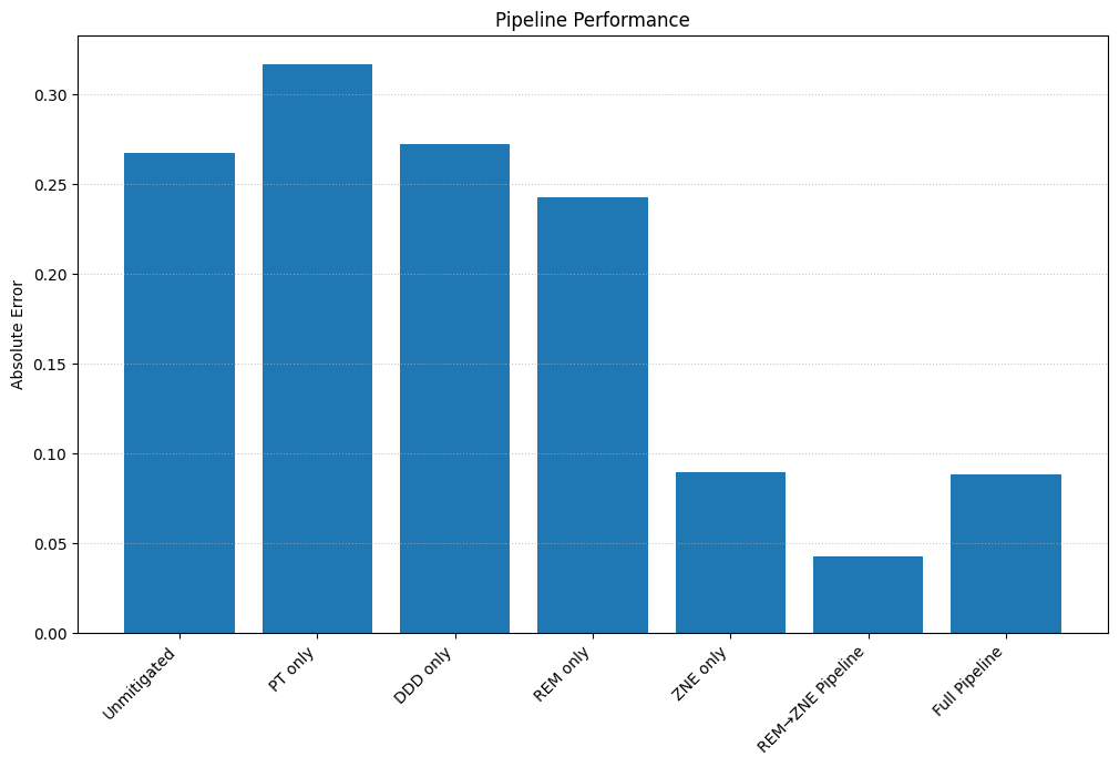
Summary of Expectation Values and Errors:
-------------------------------------------
Ideal                              : Value = +1.000000, Abs Error = 0.000000
Unmitigated                        : Value = +0.732500, Abs Error = 0.267500
PT only                            : Value = +0.683083, Abs Error = 0.316917
DDD only                           : Value = +0.728000, Abs Error = 0.272000
REM only                           : Value = +0.757250, Abs Error = 0.242750
ZNE only                           : Value = +0.910625, Abs Error = 0.089375
REM→ZNE Pipeline                   : Value = +0.957708, Abs Error = 0.042292
Full Pipeline                      : Value = +0.911861, Abs Error = 0.088139

Visually, we can see these results in a bar chart comparing errors of each method.

../_images/a1aa482f55552c68a717632742e2b96880407ae8a78744bed04787bccae49462.png

Warning

The full pipeline does not always perform best on this specific circuit and noise model.

Conclusion#

This tutorial demonstrated how to construct an advanced error mitigation pipeline by combining Pauli Twirling (PT), Digital Dynamical Decoupling (DDD), Readout Error Mitigation (REM), and Zero-Noise Extrapolation (ZNE).