Mitiq with Braket#
This notebook shows improved performance on a mirror circuit benchmark with zero-noise extrapolation on Rigetti Aspen-9 via Amazon Braket.
Note
This notebook is intended to be run through the Amazon Web Services (AWS) console — that is, by uploading the .ipynb file to https://console.aws.amazon.com/braket/ and running from there.
This requires an AWS account.
Without an AWS account, you can still run the notebook on a noisy simulator.
Setup#
import mitiq
import matplotlib.pyplot as plt
import networkx as nx
import numpy as np
import pandas as pd

from braket.aws import AwsDevice
from braket.circuits import Circuit, gates, Noise
from mitiq import benchmarks, zne
Choose a device to run on#
We first choose a device to run on.
Warning
Verbatim compiling in Braket — a necessary feature to perform zero-noise extrapolation — is currently only available on Rigetti devices.
try:
    aws_device = AwsDevice("arn:aws:braket:::device/qpu/rigetti/Aspen-9")
except:
    from braket.devices import LocalSimulator

    aws_device = LocalSimulator("braket_dm")

on_aws = aws_device.name != "DensityMatrixSimulator"
Define the circuit#
We use mirror circuits to benchmark the performance of the device. Mirror circuits, introduced in [1], are designed such that only one bitstring should be sampled. When run on a device, any other measured bitstrings are due to noise. The frequency of the correct bitstring is our target metric.
Note
Mirror circuits build on Loschmidt echo circuits — i.e., circuits of the form \(U U^\dagger\) for some unitary \(U\). Loschmidt echo circuits are good benchmarks but have shortcomings — e.g., they are unable to detect coherent errors. Mirror circuits add new features to account for these shortcomings. For more background, see https://arxiv.org/abs/2008.11294.
To define a mirror circuit, we need the device graph. We will use a subgraph of the device, and our first step is picking a subgraph with good qubits.
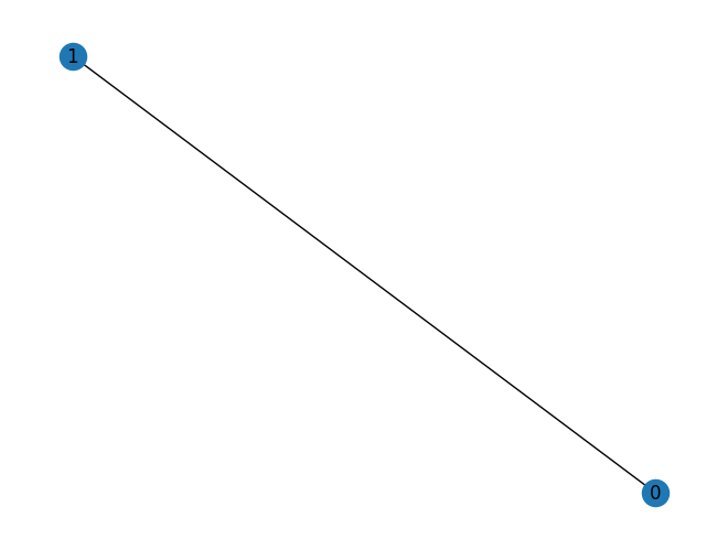
Pick good qubits#
The full device graph is shown below.
if on_aws:
    device_graph = aws_device.topology_graph
    nx.draw_kamada_kawai(device_graph, with_labels=True)
To pick good qubits, we pull the latest calibration report in the next two cells. The first cell shows two-qubit calibration data sorted by best CZ fidelity.
if on_aws:
    twoq_data = pd.DataFrame.from_dict(aws_device.properties.provider.specs["2Q"]).T

twoq_data.sort_values(by=["fCZ"], ascending=False).head() if on_aws else print()
And the next cell shows single-qubit calibration data sorted by best readout (RO) fidelity.
if on_aws:
    oneq_data = pd.DataFrame.from_dict(aws_device.properties.provider.specs["1Q"]).T

oneq_data.sort_values(by=["fRO"], ascending=False).head() if on_aws else print()
Using this calibration data as a guide, we pick good qubits and visualize the device subgraph that we will run on.
connectivity_graph = device_graph.subgraph((20, 21)) if on_aws else nx.complete_graph(2)
nx.draw(connectivity_graph, with_labels=True)
Generate mirror circuit#
Now that we have the device (sub)graph, we can generate a mirror circuit and the bitstring it should sample as follows.
circuit, correct_bitstring = benchmarks.generate_mirror_circuit(
    nlayers=1,
    two_qubit_gate_prob=1.0,
    two_qubit_gate_name="CZ",
    connectivity_graph=connectivity_graph,
    seed=1,
    return_type="braket",
)
print(circuit)
print("\nShould sample:", correct_bitstring)
T  : │     0      │     1      │     2      │     3      │     4      │     5      │  6  │  7  │  8  │  9  │ 10  │     11     │     12     │     13      │     14     │     15     │     16     │
      ┌──────────┐ ┌──────────┐ ┌──────────┐ ┌──────────┐ ┌──────────┐ ┌──────────┐ ┌───┐       ┌───┐       ┌───┐ ┌──────────┐ ┌──────────┐ ┌───────────┐ ┌──────────┐ ┌──────────┐ ┌──────────┐
q0 : ─┤ Rz(0.00) ├─┤ Ry(3.14) ├─┤ Rz(0.00) ├─┤ Rz(4.71) ├─┤ Ry(1.57) ├─┤ Rz(1.57) ├─┤ X ├───●───┤ I ├───●───┤ I ├─┤ Rz(1.57) ├─┤ Ry(1.57) ├─┤ Rz(-1.57) ├─┤ Rz(0.00) ├─┤ Ry(3.14) ├─┤ Rz(0.00) ├─
      └──────────┘ └──────────┘ └──────────┘ └──────────┘ └──────────┘ └──────────┘ └───┘   │   └───┘   │   └───┘ └──────────┘ └──────────┘ └───────────┘ └──────────┘ └──────────┘ └──────────┘
      ┌──────────┐ ┌──────────┐ ┌──────────┐ ┌──────────┐ ┌──────────┐ ┌──────────┐ ┌───┐ ┌─┴─┐ ┌───┐ ┌─┴─┐ ┌───┐ ┌──────────┐ ┌──────────┐ ┌───────────┐ ┌──────────┐ ┌──────────┐ ┌──────────┐
q1 : ─┤ Rz(6.28) ├─┤ Ry(1.57) ├─┤ Rz(0.00) ├─┤ Rz(4.71) ├─┤ Ry(1.57) ├─┤ Rz(1.57) ├─┤ X ├─┤ Z ├─┤ X ├─┤ Z ├─┤ Y ├─┤ Rz(1.57) ├─┤ Ry(1.57) ├─┤ Rz(-1.57) ├─┤ Rz(3.14) ├─┤ Ry(1.57) ├─┤ Rz(3.14) ├─
      └──────────┘ └──────────┘ └──────────┘ └──────────┘ └──────────┘ └──────────┘ └───┘ └───┘ └───┘ └───┘ └───┘ └──────────┘ └──────────┘ └───────────┘ └──────────┘ └──────────┘ └──────────┘
T  : │     0      │     1      │     2      │     3      │     4      │     5      │  6  │  7  │  8  │  9  │ 10  │     11     │     12     │     13      │     14     │     15     │     16     │

Should sample: [0, 1]
Compilation#
When using verbatim compiling on Braket, every gate must be a native hardware gate. Some single-qubit gates in the above circuit are not natively supported by Rigetti. We account for this with the quick-and-dirty compiler below.
def compile_to_rigetti_gateset(circuit: Circuit) -> Circuit:
    compiled = Circuit()

    for instr in circuit.instructions:
        if isinstance(instr.operator, gates.Vi):
            compiled.add_instruction(gates.Instruction(gates.Rx(-np.pi / 2), instr.target))
        elif isinstance(instr.operator, gates.V):
            compiled.add_instruction(gates.Instruction(gates.Rx(np.pi / 2), instr.target))
        elif isinstance(instr.operator, gates.Ry):
            compiled.add_instruction(gates.Instruction(gates.Rx(-np.pi / 2), instr.target))
            compiled.add_instruction(gates.Instruction(gates.Rz(-instr.operator.angle), instr.target))
            compiled.add_instruction(gates.Instruction(gates.Rx(np.pi / 2), instr.target))
        elif isinstance(instr.operator, gates.Y):
            compiled.add_instruction(gates.Instruction(gates.Rx(-np.pi / 2), instr.target))
            compiled.add_instruction(gates.Instruction(gates.Rz(np.pi), instr.target))
            compiled.add_instruction(gates.Instruction(gates.Rx(np.pi / 2), instr.target))
        elif isinstance(instr.operator, gates.X):
            compiled.add_instruction(gates.Instruction(gates.Rx(np.pi), instr.target))
        elif isinstance(instr.operator, gates.Z):
            compiled.add_instruction(gates.Instruction(gates.Rz(np.pi), instr.target))
        elif isinstance(instr.operator, gates.S):
            compiled.add_instruction(gates.Instruction(gates.Rz(np.pi / 2), instr.target))
        elif isinstance(instr.operator, gates.Si):
            compiled.add_instruction(gates.Instruction(gates.Rz(-np.pi / 2), instr.target))
        else:
            compiled.add_instruction(instr)

    return compiled
Define the executor#
Now that we have a circuit, we define the execute function which inputs a circuit and returns an expectation value.
In this example we return the frequency of sampling the correct bitstring.
def execute(
    circuit: Circuit,
    shots: int = 1_000,
    s3_folder: tuple[str, str] = ("bucket", "folder/"),
) -> float:
    if on_aws:
        # Add verbatim compiling so that ZNE can be used.
        circuit = Circuit().add_verbatim_box(
            compile_to_rigetti_gateset(circuit)
        )

        aws_task = aws_device.run(
            circuit, s3_folder, disable_qubit_rewiring=True, shots=shots
        )

    else:
        aws_task = aws_device.run(
            circuit.copy().apply_gate_noise(
                Noise.Depolarizing(probability=0.002)
            ),
            shots=shots,
        )

    return aws_task.result().measurement_probabilities.get(
        "".join(map(str, correct_bitstring)), 0.0
    )
Noisy value#
The result of running the example mirror circuit without zero-noise extrapolation is shown below.
noisy_value = execute(circuit)
print("Noisy value:", noisy_value)
Noisy value: 0.958
Mitigated value#
The result of running the example mirror circuit with zero-noise extrapolation is shown below.
zne_value = zne.execute_with_zne(
    circuit,
    execute,
    scale_noise=zne.scaling.fold_global,
    factory=zne.inference.PolyFactory(scale_factors=[1, 3, 5], order=2)
)
print("ZNE value:", zne_value)
ZNE value: 0.9820000000000002
In this simple example, we see that zero-noise extrapolation improves the result. (Recall that the noiseless value is 1.0.)
Survival probability vs. depth#
Now we run the same experiment above but varying the depth (nlayers) of the mirror circuit. We also average over several mirror circuits at each depth.
# Experiment parameters.
nlayers_values = list(range(1, 20, 2))
ntrials = 4

# To store results.
noisy_values = []
zne_values = []

# Run the experiment and store results.
for nlayers in nlayers_values:
    for i in range(ntrials):
        circuit, correct_bitstring = benchmarks.generate_mirror_circuit(
            nlayers=nlayers,
            two_qubit_gate_prob=1.0,
            two_qubit_gate_name="CZ",
            connectivity_graph=connectivity_graph,
            seed=i,
            return_type="braket",
        )

        noisy_values.append(execute(circuit))
        zne_values.append(
            zne.execute_with_zne(
                circuit,
                execute,
                scale_noise=zne.scaling.fold_global,
                factory=zne.inference.PolyFactory(scale_factors=[1, 3, 5], order=2)),
        )
Now we can visualize the results.
average_zne_values = np.average(np.array(zne_values).reshape((len(nlayers_values), ntrials)), axis=1)
average_noisy_values = np.average(np.array(noisy_values).reshape((len(nlayers_values), ntrials)), axis=1)

plt.rcParams.update({"font.family": "serif", "font.size": 16})
plt.figure(figsize=(9, 5))

plt.plot(nlayers_values, average_zne_values, "--o", label="ZNE")
plt.plot(nlayers_values, average_noisy_values, "-.o", label="Raw")

plt.xlabel("Circuit depth")
plt.ylabel("Survival probability")

plt.legend()
plt.show();
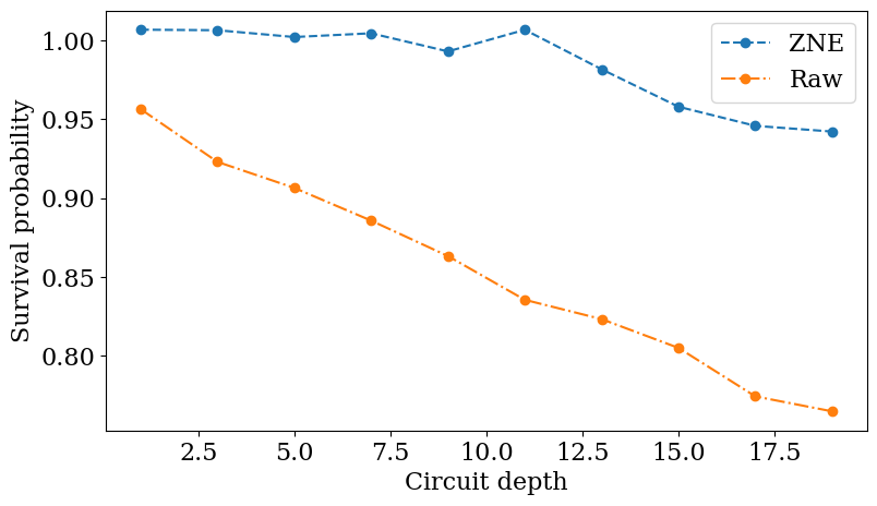
We see that zero-noise extrapolation on average improves the survival probability at each depth.