Learning quasiprobability representations with a depolarizing noise model#
In this example, we demonstrate the workflow of learning quasiprobability representations of a CNOT gate with a depolarizing noise model,
from Clifford circuit data.
The depolarizing noise model is parameterized by the noise strength, epsilon.
The resulting quasiprobability representations of the CNOT gate are then used to obtain an error-mitigated expectation value with Mitiq’s
probabilistic error cancellation module.
For a more in-depth description of the learning function used in this example, see the section on learn_depolarizing_noise_parameter()
in the API-doc.
The learning-based PEC workflow was inspired by the procedure described in Strikis et al. PRX Quantum (2021) [16].
import numpy as np
from matplotlib import pyplot as plt
from cirq import (
    CXPowGate,
    DepolarizingChannel,
    LineQubit,
    Circuit,
)
from mitiq import Executor, Observable, PauliString
from mitiq.interface.mitiq_cirq import compute_density_matrix
from mitiq.cdr import generate_training_circuits
from mitiq.cdr._testing import random_x_z_cnot_circuit
from mitiq.pec import execute_with_pec
from mitiq.pec.representations.depolarizing import (
    represent_operation_with_local_depolarizing_noise,
)
from mitiq.pec.representations.learning import (
    depolarizing_noise_loss_function,
    learn_depolarizing_noise_parameter,
)
Since the learning-based workflow uses the function cdr.clifford_training_data.generate_training_circuits() from Mitiq’s Clifford data regression module to generate the near-Clifford training circuits, the input circuit must be one that is compiled into the Rx-Rz-CNOT gateset.
Here we use a simple Rx-Rz-CNOT circuit, with an (optional) seed for reproducibility.
circuit = random_x_z_cnot_circuit(
    LineQubit.range(2), n_moments=5, random_state=np.random.RandomState(1)
)
print(circuit)
0: ───Rx(1.14π)───Rz(0)───X───Rx(1.71π)───────────────
                          │
1: ───────────────────────@───────────────Rx(1.14π)───
Define the ideal executor function for simulating the Clifford training circuits without noise. This will be used for comparison to the error-mitigated expectation values in the learning function, and for a final comparison with the mitigated and unmitigated values at the end of the workflow.
def ideal_execute(circ: Circuit) -> np.ndarray:
    # For large circuits, this should be replaced by a near-Clifford simulator.
    return compute_density_matrix(circ, noise_level=(0.0,))


ideal_executor = Executor(ideal_execute)
Define the noisy executor, in this case for simulating depolarizing noise on the CNOT gate in each of the training circuits.
The optimized value of the noise strength epsilon should be close to the value defined for this executor.
CNOT_ops = list(circuit.findall_operations_with_gate_type(CXPowGate))

operations_to_learn = [Circuit(op[1]) for op in CNOT_ops]

epsilon = 0.05

def noisy_execute(circ: Circuit) -> np.ndarray:
    noisy_circ = circ.copy()
    insertions = []
    for op in CNOT_ops:
        index = op[0] + 1
        qubits = op[1].qubits
        for q in qubits:
            insertions.append((index, DepolarizingChannel(epsilon)(q)))
    noisy_circ.batch_insert(insertions)

    return ideal_execute(noisy_circ)


noisy_executor = Executor(noisy_execute)
Before calling the optimizer, let’s plot the loss function that will be minimized in the learning routine, over a small range of noise strength values.
The loss function calls pec.execute_with_pec(), and we can optionally pass keyword arguments to set the number of PEC samples, among other options.
Here we set a relatively small value of num_samples to obtain a reasonable execution time.
However, we avoid using a number of PEC samples that is too small, as it can result in a large statistical error and ultimately cause the optimization process to fail.
pec_kwargs = {"num_samples": 500, "random_state": 1}
observable = Observable(PauliString("XZ"), PauliString("YY"))

import warnings
# suppress warnings about missing representations
# this example only simulates noise on CNOT
warnings.simplefilter("ignore", UserWarning)
training_circuits = generate_training_circuits(
    circuit=circuit,
    num_training_circuits=5,
    fraction_non_clifford=0.2,
    random_state=np.random.RandomState(1),
)

ideal_values = np.array(ideal_executor.evaluate(training_circuits, observable))

epsilons = np.linspace(0.03, 0.07, 9)

loss = [
    depolarizing_noise_loss_function(
        [eps],
        operations_to_learn,
        training_circuits,
        ideal_values,
        noisy_executor,
        pec_kwargs,
        observable=observable,
    )
    for eps in epsilons
]

_ = plt.plot(epsilons, loss)
plt.title("Depolarizing noise loss function")
plt.xlabel("Noise strength")
plt.ylabel("Loss")
plt.show()
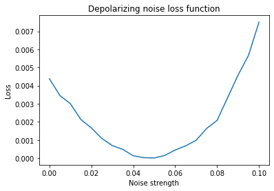
The figure is a plot of the loss function for optimizing quasi-probability representations assuming a depolarizing noise model depending on one real parameter.#
Now we set the initial conditions for the optimization. For purposes of this demonstration, our initial guess for epsilon, epsilon0, is
slightly offset from the true value of epsilon.
offset = 0.1
epsilon0 = (1 - offset) * epsilon
Here we use the Nelder-Mead method in scipy.optimize.minimize
to find the value of epsilon that minimizes the depolarizing noise loss function.
[success, epsilon_opt] = learn_depolarizing_noise_parameter(
    operations_to_learn,
    circuit,
    ideal_executor,
    noisy_executor,
    pec_kwargs,
    num_training_circuits=5,
    fraction_non_clifford=0.2,
    training_random_state=np.random.RandomState(1),
    epsilon0=epsilon0,
    observable=observable,
)
print(success)
print(f"Difference of learned value from true value: {abs(epsilon_opt - epsilon) :.5f}")
print(f"Difference of initial guess from true value: {abs(epsilon0 - epsilon) :.5f}")
True
Difference of learned value from true value: 0.00050
Difference of initial guess from true value: 0.00500
Optimization completed successfully and the optimized value of epsilon is closer to the true value of epsilon as compared to the initial value.
Now we will use the optimized value of the noise strength to map CNOT into its quasiprobability representation.
representations = [
    represent_operation_with_local_depolarizing_noise(op, epsilon_opt)
    for op in operations_to_learn
]
Apply PEC on original noisy circuit to obtain the error-mitigated expectation value.
mitigated = execute_with_pec(
    circuit=circuit,
    executor=noisy_executor,
    observable=observable,
    representations=representations,
    **pec_kwargs,
)
mitigated_result = mitigated.real
print(f"Error-mitigated result with learning-based PEC: {mitigated_result:.5f}")
Error-mitigated result with learning-based PEC: -0.18565
Comparing with unmitigated and ideal values, we see that the mitigated value, calculated with the learned depolarizing noise strength, is closer to the ideal value, as compared with the noisy value.
noisy_value = noisy_executor.evaluate(circuit, observable)[0].real
ideal_value = ideal_executor.evaluate(circuit, observable)[0].real
print(f"Error without mitigation: {abs(ideal_value - noisy_value) :.5f}")
print(f"Error with mitigation (PEC): {abs(ideal_value - mitigated_result):.{3}}")
Error without mitigation: 0.02426
Error with mitigation (PEC): 0.0026