Mitigating the energy landscape of a variational circuit with Mitiq and PennyLane

This tutorial shows an example in which the energy landscape for a two-qubit variational circuit is explored using the PennyLane frontend, with and without error mitigation in Mitiq.

import matplotlib.pyplot as plt
import pennylane as qml
import pennylane_qiskit
from pennylane import numpy as np

from mitiq.zne import mitigate_executor
from mitiq.zne.inference import RichardsonFactory
from mitiq.zne.scaling import fold_global as folding

Defining the ideal variational circuit in PennyLane

We define a function which returns a simple two-qubit variational circuit depending on a single parameter \(\gamma\) (“gamma”).

noise_strength = 0.04

# Ideal device
dev = qml.device("default.mixed", wires=2)
# noisy device
dev_noisy = qml.transforms.insert(dev, qml.DepolarizingChannel, noise_strength)

def variational_circuit(gamma: float):
    """Returns a two-qubit circuit for a given variational parameter.

    Args:
        gamma: The variational parameter.

    Returns:
        The two-qubit circuit with a fixed gamma.
    """
    qml.RX(gamma, wires=0)
    qml.CNOT(wires=[0,1])
    qml.RX(gamma, wires=1)
    qml.CNOT(wires=[0, 1])
    qml.RX(gamma, wires=0)

We can visualize the circuit for a particular \(\gamma\) as follows.

drawer = qml.draw(variational_circuit)
print(drawer(np.pi))

0: ──RX(3.14)─╭●───────────╭●──RX(3.14)─┤  
1: ───────────╰X──RX(3.14)─╰X───────────┤  

Defining the executor functions with and without noise

To use error mitigation methods in Mitiq, we define an executor function which computes the expectation value of a simple Hamiltonian \(H=Z \otimes Z\), i.e., Pauli-\(Z\) on each qubit. To compare to the noiseless result, we define both a noiseless and a noisy executor below.

# Observable to measure
z = np.diag([1, -1])
hamiltonian = np.kron(z, z)

@qml.qnode(dev)#using ideal simulator
def noiseless_executor(gamma) -> float:
    """Simulates the execution of a circuit without noise.

    Args:
        gamma: parameter.

    Returns:
        The expectation value of the ZZ observable.
    """
    variational_circuit(gamma)
    return qml.density_matrix([1,0])


@qml.qnode(dev_noisy)#using noisy simulator
def executor_with_noise(gamma) -> float:
    """Simulates the execution of a circuit with depolarizing noise.

    Args:
        gamma: parameter.

    Returns:
        The expectation value of the ZZ observable.
    """
    variational_circuit(gamma)
    return qml.density_matrix([1,0])

The above code block uses depolarizing noise, but any PennyLane Channel (noise model) can be substituted in.

Computing the landscape without noise

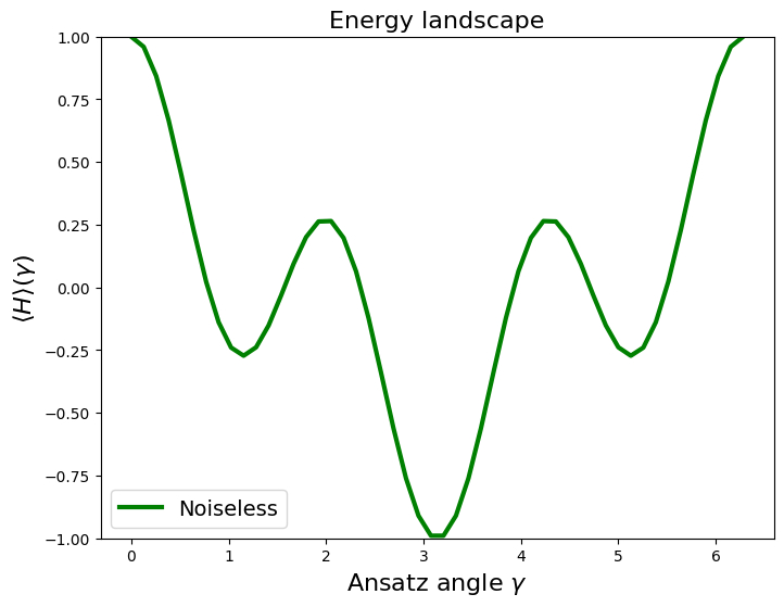
We now compute the energy landscape \(\langle H \rangle(\gamma) =\langle Z \otimes Z \rangle(\gamma)\) on the noiseless simulator. The remaining code in this tutorial is generic and does not depend on a particular frontend.

gammas = np.linspace(0, 2 * np.pi, 50)
noiseless_expectations = [np.real(np.trace(noiseless_executor(g)@ hamiltonian)) for g in gammas]

plt.figure(figsize=(8, 6))
plt.plot(gammas, noiseless_expectations, color="g", linewidth=3, label="Noiseless")
plt.title("Energy landscape", fontsize=16)
plt.xlabel(r"Ansatz angle $\gamma$", fontsize=16)
plt.ylabel(r"$\langle H \rangle(\gamma)$", fontsize=16)
plt.legend(fontsize=14)
plt.ylim(-1, 1);
plt.show()

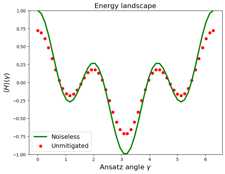
Computing the unmitigated landscape

We now compute the unmitigated energy landscape \(\langle H \rangle(\gamma) =\langle Z \otimes Z \rangle(\gamma)\) in the following code block.

gammas = np.linspace(0, 2 * np.pi, 50)
expectations = [np.real(np.trace(executor_with_noise(g)@ hamiltonian)) for g in gammas]

The following code plots these values for visualization along with the noiseless landscape.

plt.figure(figsize=(8, 6))
plt.plot(gammas, noiseless_expectations, color="g", linewidth=3, label="Noiseless")
plt.scatter(gammas, expectations, color="r", label="Unmitigated")
plt.title(rf"Energy landscape", fontsize=16)
plt.xlabel(r"Ansatz angle $\gamma$", fontsize=16)
plt.ylabel(r"$\langle H \rangle(\gamma)$", fontsize=16)
plt.legend(fontsize=14)
plt.ylim(-1, 1);
plt.show()

Computing the mitigated landscape

We now repeat the same task but use Mitiq to mitigate errors. We initialize a RichardsonFactory with scale factors [1, 3, 5] and we get a mitigated executor as follows.

extrapolate = RichardsonFactory.extrapolate
scale_factors = [1, 3, 5]
@qml.qnode(dev_noisy)
def circuit(gamma: float):
    """Returns a two-qubit circuit for a given variational parameter.

    Args:
        gamma: The variational parameter.

    Returns:
        The two-qubit circuit with a fixed gamma.
    """
    variational_circuit(gamma)
    return qml.expval(qml.PauliZ(0) @ qml.PauliZ(1))

circuit = qml.transforms.mitigate_with_zne(circuit, scale_factors, folding, extrapolate)

We then run the same code above to compute the energy landscape, but this time use the mitigated executor.

mitigated_expectations = [circuit(g) for g in gammas]

Let us visualize the mitigated landscape alongside the unmitigated and noiseless landscapes.

plt.figure(figsize=(8, 6))
plt.plot(gammas, noiseless_expectations, color="g", linewidth=3, label="Noiseless")
plt.scatter(gammas, expectations, color="r", label="Unmitigated")
plt.scatter(gammas, mitigated_expectations, color="b", label="Mitigated")
plt.title(rf"Energy landscape", fontsize=16)
plt.xlabel(r"Variational angle $\gamma$", fontsize=16)
plt.ylabel(r"$\langle H \rangle(\gamma)$", fontsize=16)
plt.legend(fontsize=14)
plt.ylim(-1.5, 1.5);
plt.show()

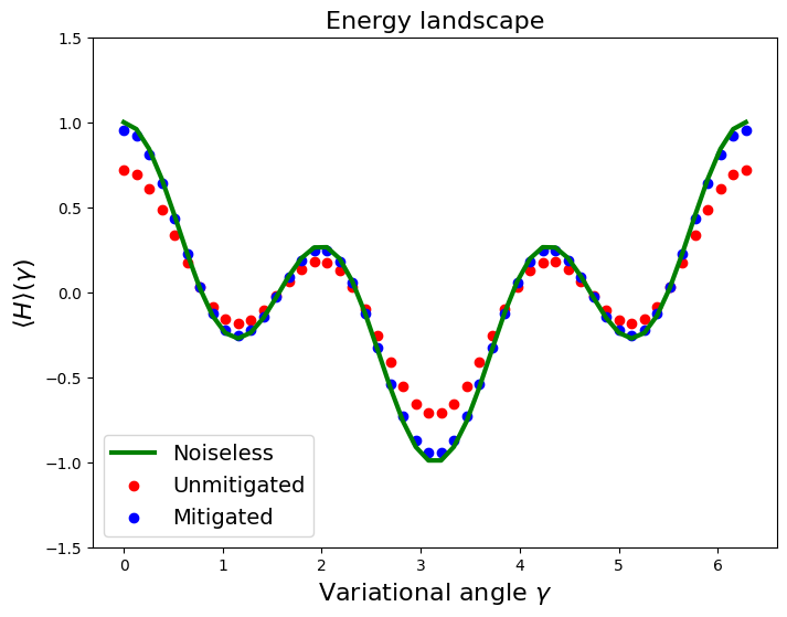
Noise usually tends to flatten expectation values towards a constant. Therefore error mitigation can be used to increase the visibility the landscape and this fact can simplify the energy minimization which is required in most variational algorithms such as VQE or QAOA.

We also observe that the minimum of mitigated energy approximates well the theoretical ground state which is equal to \(-1\). Indeed:

print(f"Minimum of the noisy landscape: {round(min(expectations), 3)}")
print(f"Minimum of the mitigated landscape: {round(min(mitigated_expectations), 3)}")
print(f"Theoretical ground state energy: {min(np.linalg.eigvals(hamiltonian))}")

Minimum of the noisy landscape: -0.713
Minimum of the mitigated landscape: -0.946
Theoretical ground state energy: -1.0