Probabilistic error cancellation (PEC) with Mirror Circuits

This notebook shows probabilistic error cancellation (PEC) Temme et al. PRL (2017) [5], Sun et al. PRLAppl (2021) [10], Zhang et al. NatComm (2020) [48], improving performance of a mirror circuit benchmark on the braket_dm noisy simulator.

In PEC, the first step is to characterize the set of noisy, implementable operations \(\{\mathcal{O_{\alpha}}\}\) of a quantum device so that we can represent the ideal (noiseless) operations \(\{\mathcal{G}_i\}\) of a circuit in this basis, namely

\[ \mathcal{G}_i = \sum_{\alpha} \eta_{i, \alpha} \mathcal{O}_{\alpha}. \]

Note that the calligraphic symbols \(\mathcal{G}_i\) and \(\mathcal{O}_{\alpha}\) stand for super-operators acting on the quantum state of the qubits as linear quantum channels, and \(\eta_{i, \alpha} \in \mathbb{R}\).

Setup

We begin by importing the relevant modules and libraries that we will require for the rest of this tutorial.

import functools
from typing import List, Tuple, Union

# Plotting imports.
import matplotlib.pyplot as plt
plt.rcParams.update({"font.family": "serif", "font.size": 15})
%matplotlib inline

# Third-party imports.
import cirq
import qiskit

import networkx as nx
import numpy as np

from braket.devices import LocalSimulator
from braket.circuits import Circuit, gates, Noise

# Mitiq imports.
from mitiq import benchmarks, pec

import warnings
warnings.filterwarnings('ignore')

Define parameters

# Random seed for circuit generation.
seed: int = 1               

# Total number of shots to use.
# For PEC, the shots per circuit is shots / num_samples.
shots: int = 10_000     

# Number of samples (circuits) to use in PEC.    
num_samples: int = 100  
    
# Qubits to use on the experiment. 
qubits: List[int] = [0, 1, 2]
        
# Average results over this many trials (circuit instances) at each depth.
trials: int = 4      
    
# As operating on simulator, assume a constant CNOT error rate.
cnot_error_prob: float = 0.01

# Clifford depths.
depths: List[int] = [1, 5, 9]

Next, we need to define both the noisy and ideal simulator backends that we will run our experiments on. In this case, we will be making use of the braket_dm simulator.

We also define a graph representation of our qubits and assume a line topology.

# Assume chain-like connectivity
computer = nx.Graph()
computer.add_edges_from([(0, 1), (1, 2)])

# Add reversed edges to computer graph.
# This is important to represent CNOT gates with target and control reversed.
computer = nx.to_directed(computer)

noisy_backend = LocalSimulator("braket_dm")
ideal_backend = LocalSimulator("default")

Define the circuit

We use mirror circuits to benchmark the performance of the device. Mirror circuits, introduced in Proctor et al. arXiv (2021) [56] (arXiv:2008.11294), are designed such that only one bitstring should be sampled. When run on a device, any other measured bitstrings are due to noise. The frequency of the correct bitstring is our target metric.

Note

Mirror circuits build on Loschmidt echo circuits — i.e., circuits of the form \(U U^\dagger\) for some unitary \(U\). Loschmidt echo circuits are good benchmarks but have shortcomings — e.g., they are unable to detect coherent errors. Mirror circuits add new features to account for these shortcomings. For more background, see arXiv:2008.11294.

To define a mirror circuit, we need the device graph. We will use a subgraph of the device, and our first step is picking a subgraph with good qubits.

Generate mirror circuit

Now that we have the device (sub)graph, we can generate a mirror circuit and the bitstring it should sample as follows.

def get_circuit(depth: int, seed: int) -> Union[Tuple[cirq.Circuit, str], Tuple[qiskit.QuantumCircuit, str]]:
    circuit, correct_bitstring = benchmarks.generate_mirror_circuit(
        nlayers=depth,
        two_qubit_gate_prob=1.0,
        connectivity_graph=computer,
        two_qubit_gate_name="CNOT",
        seed=seed,
        return_type="braket",
    )        
    return circuit, correct_bitstring 

PEC representations

PEC makes use of quasi-probability representations. We define these here in terms of CNOT operations. For more information about these representations in the context of PEC and usage within mitiq, refer to the What is the theory behind PEC? page.

def get_cnot_representation(edge: Tuple[int, int]) -> pec.OperationRepresentation:
    cnot_circuit = cirq.Circuit(cirq.CNOT(cirq.LineQubit(edge[0]), cirq.LineQubit(edge[1])))              
    
    rep_exact_prob = 1 - np.sqrt(1 - cnot_error_prob)
    return pec.represent_operation_with_local_depolarizing_noise(
        cnot_circuit, 
        noise_level=rep_exact_prob,
    )


def get_representations(computer: nx.Graph) -> List[pec.OperationRepresentation]:
    return [get_cnot_representation(edge) for edge in computer.edges]

Helper methods

It will be useful later to us to have a number of utility functions for counting CNOT gates and operations.

def get_num_cnot_count(circuit: Union[cirq.Circuit, qiskit.QuantumCircuit]) -> int:
    """Determine number of cnot gates in a given `Circuit` object."""    
    # Count CNOT gates for `cirq`-type circuit objects:
    num_cnots: int = 0
    for instruction in circuit.instructions:
        if isinstance(instruction.operator, gates.CNot):
            num_cnots += 1
    return num_cnots

def get_oneq_count(circuit: Union[cirq.Circuit, qiskit.QuantumCircuit]) -> int:
    return len(circuit.instructions) - get_num_cnot_count(circuit)

Define the executor

Now that we have a circuit, we define the execute function which inputs a circuit and returns an expectation value - here, the frequency of sampling the correct bitstring.

def execute(
    circuits: Union[cirq.Circuit, List[cirq.Circuit]], 
    backend,
    shots: int,
    correct_bitstring: str,
    is_noisy: bool = True,
) -> List[float]:
    """Executes the input circuit(s) and returns ⟨A⟩, where 
    A = |correct_bitstring⟩⟨correct_bitstring| for each circuit.
    """
    if not isinstance(circuits, list):
        circuits = [circuits]
    
    # Store all circuits to run in list to be returned.
    to_run: Union[List[braket.Circuit], List[qiskit.QuantumCircuit]] = []
    
    # Compile circuits to appropriate gateset.
    for circuit in circuits:
        circuit_to_run = circuit.copy()            
        if is_noisy:            
            circuit_to_run.apply_gate_noise(
                Noise.Depolarizing(probability=cnot_error_prob/2), target_gates=gates.CNot
            )
        to_run.append(circuit_to_run)
        
    # Process each job.
    results: List[float] = []
    for circ_to_run in to_run:
        job_result = backend.run(circ_to_run, shots=shots).result()
        results.append(job_result.measurement_probabilities.get("".join(map(str, correct_bitstring)), 0.0))

    return results

Running the experiment

PEC samples many circuits according to the input representations. Each unitary gate \(U\) in the circuit, with representation

\[ U = \sum_i a_i G_i, \]

is replaced by \(G_i\) with probability \(|a_i| /\gamma\), where \(\gamma=\sum_i |a_i|\).

This procedure is repeated multiple times, generating \(M\) (num_samples) circuits. The associated noisy expectation values are re-combined by Mitiq according to the following formula

\[ \frac{\gamma}{M} \sum_{i=1}^M {\rm sign}(a_i) E_i , \]

which is an unbiased estimator of the true (noiseless) expectation value.

cnot_counts, oneq_counts = [], []
true_values, noisy_values = [], []
pec_values = []

noise_scaled_expectation_values = []

for depth in depths:
    print("Status: On depth", depth, end="\n\n")
    
    cnot_depth_counts, oneq_depth_counts = [], []
    true_depth_values, noisy_depth_values = [], []
    pec_depth_values = []

    noise_scaled_expectation_depth_values = []

    for trial in range(trials):
        # Local seed is calculated in this way to ensure that we don't get repeat values in loop.        
        local_seed = 10**6 * depth + 10**3 * seed + trial
        
        circuit, correct_bitstring = get_circuit(depth, local_seed)

        true_value, = execute(circuit, ideal_backend, shots, correct_bitstring, is_noisy=False)
        noisy_value, = execute(circuit, noisy_backend, shots, correct_bitstring, is_noisy=True)
        
        pec_executor = functools.partial(
            execute, 
            backend=noisy_backend, 
            shots=shots // num_samples,
            correct_bitstring=correct_bitstring,
        )
        
        pec_value = pec.execute_with_pec(
            circuit, 
            pec_executor, 
            representations=get_representations(computer), 
            num_samples=num_samples,
            random_state=local_seed,
        )

        pec_depth_values.append(pec_value)

        cnot_depth_counts.append(get_num_cnot_count(circuit))
        oneq_depth_counts.append(get_oneq_count(circuit))
        
        true_depth_values.append(true_value)
        noisy_depth_values.append(noisy_value)
    
    cnot_counts.append(cnot_depth_counts)
    oneq_counts.append(oneq_depth_counts)
    
    true_values.append(true_depth_values)
    noisy_values.append(noisy_depth_values)
    
    noise_scaled_expectation_values.append(noise_scaled_expectation_depth_values)    
    
    pec_values.append(pec_depth_values)

Status: On depth 1

Status: On depth 5

Status: On depth 9

Now we can visualize the results.

avg_true_values = np.average(true_values, axis=1)
avg_noisy_values = np.average(noisy_values, axis=1)

std_true_values = np.std(true_values, axis=1, ddof=1)
std_noisy_values = np.std(noisy_values, axis=1, ddof=1)

avg_pec_values = np.average(pec_values, axis=1)
std_pec_values = np.std(pec_values, axis=1, ddof=1)

plt.figure(figsize=(9, 5))

plt.plot(depths, avg_true_values,  '--', label="True", lw=2)
eb = plt.errorbar(depths, avg_noisy_values, yerr=std_noisy_values, label="Raw", ls='-.')
eb[-1][0].set_linestyle('-.')
plt.errorbar(depths, avg_pec_values, yerr=std_pec_values, label="PEC")
    
plt.title(f"""Simulator with mirror circuits using PEC \nqubits {qubits}, {trials} trials.""")
plt.xlabel("Depth")
plt.ylabel("Expectation value")
plt.legend();

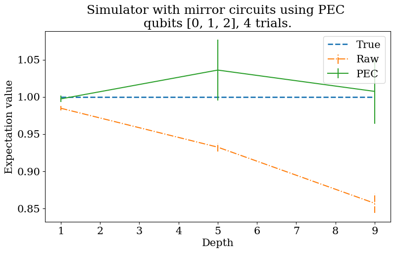
We can see that PEC on average improves the expectation value at each depth. Note that the size of the error bars represents the standard deviation of the noisy values (for the “Raw” line) and the standard deviation of the PEC values (for the “PEC” line).

For an example of how one applies PEC on quantum hardware consult Russo et al. arXiv (2022) [70] (arXiv:2210.07194) and the companion software repository.