Defining Hamiltonians as Linear Combinations of Pauli Strings

This tutorial shows an example of using Hamiltonians defined as PauliSum objects or similar objects in other supported frontends. The usage of these Hamiltonian-like objects does not change the interface with Mitiq, but we show an example for users who prefer these constructions.

Specifically, in this tutorial we will mitigate the expectation value of the following Hamiltonian on two qubits.

\[ H := 1.5 X_1 Z_2 - 0.7 Y_1 \]

Setup

First we import libraries for this example.

from functools import partial

import matplotlib.pyplot as plt
import numpy as np

import cirq
from mitiq.zne import execute_with_zne
from mitiq.zne.inference import LinearFactory

Defining the Hamiltonian

Now we define the Hamiltonian as a PauliSum by defining the Pauli strings \(X_1 Z_2\) and \(Y_1\) then taking a linear combination of these to create the Hamiltonian above.

# Qubit register
qreg = cirq.LineQubit.range(2)

# Two Pauli operators
string1 = cirq.PauliString(cirq.ops.X.on(qreg[0]), cirq.ops.Z.on(qreg[1]))
string2 = cirq.PauliString(cirq.ops.Y.on(qreg[1]))

# Hamiltonian
ham = 1.5 * string1 - 0.7 * string2

By printing the Hamiltonian we see:

print(ham)

1.500*X(q(0))*Z(q(1))-0.700*Y(q(1))

Note that we could have created the Hamiltonian by directly defining a PauliSum with the coefficients.

Using the Hamiltonian in the executor

To interface with Mitiq, we define an executor function which maps an input (noisy) circuit to an expectation value. In the code block below, we show how to define this function and return the expectation of the Hamiltonian above.

def executor(
    circuit: cirq.Circuit, hamiltonian: cirq.PauliSum, noise_value: float
) -> float:
    """Runs the circuit and returns the expectation value of the Hamiltonian.

    Args:
        circuit: Defines the ansatz wavefunction.
        hamiltonian: Hamiltonian to compute the expectation value of w.r.t. the ansatz wavefunction.
        noise_value: Probability of depolarizing noise.
    """
    # Add noise
    noisy_circuit = circuit.with_noise(cirq.depolarize(noise_value))

    # Get the final density matrix
    dmat = (
        cirq.DensityMatrixSimulator()
        .simulate(noisy_circuit)
        .final_density_matrix
    )

    # Return the expectation value
    return hamiltonian.expectation_from_density_matrix(
        dmat, qubit_map={ham.qubits[i]: i for i in range(len(ham.qubits))}
    ).real

This executor inputs a Hamiltonian as well as a noise value, adds noise, then uses the cirq.PauliSum.expectation_from_density_matrix() method to return the expectation value.

The remaining interface is as usual with Mitiq. For the sake of example, we show an application mitigating the expectation value of \(H\) with an example ansatz at different noise levels.

Example usage

Below we create an example ansatz parameterized by one angle \(\gamma\).

def ansatz(gamma: float) -> cirq.Circuit:
    """Returns the ansatz circuit."""
    return cirq.Circuit(
        cirq.ops.ry(gamma).on(qreg[0]),
        cirq.ops.CNOT.on(*qreg),
        cirq.ops.rx(gamma / 2).on_each(qreg),
        cirq.ops.CNOT.on(*qreg),
    )

For the angle \(\gamma = \pi\), this ansatz has the following structure:

print(ansatz(gamma=np.pi))

0: ───Ry(π)───@───Rx(0.5π)───@───
              │              │
1: ───────────X───Rx(0.5π)───X───

We now compute expectation values of \(H\) using the executor as follows.

pvals = np.linspace(0, 0.01, 20)
expvals = [executor(ansatz(gamma=np.pi), ham, p) for p in pvals]

We can compute mitigated expectation values at these same noise levels by running the following. Here, we use a LinearFactory and use the partial function to update the executor for each noise value. The latter point ensures this_executor has the correct signature (input circuit, output float) to use with execute_with_zne().

fac = LinearFactory(scale_factors=list(range(1, 6)))
mitigated_expvals = []

for p in pvals:
    this_executor = partial(executor, hamiltonian=ham, noise_value=p)
    mitigated_expvals.append(
        execute_with_zne(ansatz(gamma=np.pi), this_executor, factory=fac)
    )

We can now visualize the effect that error mitigation has by running the following code for plotting. This produces a plot of expectation value (unmitigated and mitigated) \(\langle H \rangle\) vs. noise strength \(p\). We include the true (noiseless) expectation value on the plot for comparison.

plt.rcParams.update({"font.family": "serif", "font.size": 16})
plt.figure(figsize=(9, 5))

plt.axhline(y=expvals[0], label="True", color="black")
plt.plot(pvals, expvals, "--o", label="Unmitigated")
plt.plot(pvals, mitigated_expvals, "-.o", label="Mitigated")

plt.xlabel("Noise strength $p$")
plt.ylabel(r"Expecation value $\langle H \rangle$")
plt.legend()
plt.show()

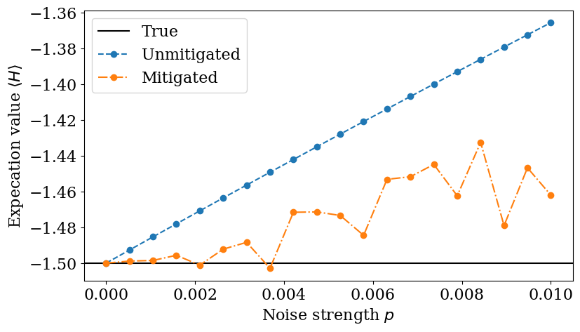
As we can see, the mitigated expectation values are closer, on average, to the true expectation value.

Sampling

Finally, we note that \(\langle H \rangle\) can be estimated by sampling using the cirq.PauliSumCollector. An example of a sampling_executor which uses this is shown below.

def sampling_executor(
    circuit: cirq.Circuit,
    hamiltonian: cirq.PauliSum,
    noise_value: float,
    nsamples: int = 10_000
) -> float:
    """Runs the circuit and returns the expectation value of the Hamiltonian.

    Args:
        circuit: Defines the ansatz wavefunction.
        hamiltonian: Hamiltonian to compute the expectation value of w.r.t. the ansatz wavefunction.
        noise_value: Probability of depolarizing noise.
        nsamples: Number of samples to take per each term of the Hamiltonian.
    """
    # Add noise
    noisy_circuit = circuit.with_noise(cirq.depolarize(noise_value))

    # Do the sampling
    psum = cirq.PauliSumCollector(circuit, ham, samples_per_term=nsamples)
    psum.collect(sampler=cirq.Simulator())

    # Return the expectation value
    return psum.estimated_energy()

This executor can be used in the same way as the previously defined executor which used a density matrix simulation to evaluate \(\langle H \rangle\).